Aufgaben:Exercise 4.16: Eigenvalues and Eigenvectors: Difference between revisions

From LNTwww
Nabil (talk | contribs)
No edit summary
Fix interlanguage link: resolve redirect chain
 
(24 intermediate revisions by 5 users not shown)
Line 1: Line 1:


{{quiz-Header|Buchseite=Stochastische Signaltheorie/Verallgemeinerung auf N-dimensionale Zufallsgrößen
{{quiz-Header|Buchseite=Theory_of_Stochastic_Signals/Generalization_to_N-Dimensional_Random_Variables
}}
}}


[[File:P_ID671__Sto_A_4_16.png|right|]]
[[File:P_ID671__Sto_A_4_16.png|right|frame|Three correlation matrices]]
:Obwohl die Beschreibung Gaußscher Zufallsgrößen mit Hilfe von Vektoren und Matrizen eigentlich nur bei mehr als <i>N</i> = 2 Dimensionen erforderlich ist und Sinn macht, beschränken wir uns hier auf den Sonderfall zweidimensionaler Zufallsgrößen.
Although the description of Gaussian random variables using vectors and matrices is actually only necessary and makes sense for more than&nbsp; $N = 2$&nbsp; dimensions,&nbsp; here we restrict ourselves to the special case of two-dimensional random variables for simplicity.


:In der Grafik ist oben die allgemeine Korrelationsmatrix <b>K<sub>x</sub></b> der 2D&ndash;Zufallsgröße <b>x</b> = (<i>x</i><sub>1</sub>, <i>x</i><sub>2</sub>)<sup>T</sup> angegeben, wobei <i>&sigma;</i><sub>1</sub><sup>2</sup> und <i>&sigma;</i><sub>2</sub><sup>2</sup> die Varianzen der Einzelkomponenten beschreiben. <i>&rho;</i> bezeichnet den Korrelationskoeffizienten zwischen den beiden Komponenten.
In the graph above,&nbsp; the general correlation matrix&nbsp; $\mathbf{K_x}$&nbsp; of the two-dimensional random variable &nbsp; $\mathbf{x} = (x_1, x_2)^{\rm T}$ &nbsp; is given,&nbsp; where&nbsp; $\sigma_1^2$&nbsp; and&nbsp; $\sigma_2^2$&nbsp; describe the variances of the individual components. &nbsp; $\rho$&nbsp; denotes the correlation coefficient between the two components.


:Die Zufallsgrößen <b>y</b> und <b>z</b> geben zwei Spezialfälle von <b>x</b> an, deren Prozessparameter aus den Kovarianzmatrizen <b>K<sub>y</sub></b> und <b>K<sub>z</sub></b> bestimmt werden können.<br>
The random variables &nbsp; $\mathbf{y}$ &nbsp; and &nbsp; $\mathbf{z}$ &nbsp; give two special cases of&nbsp; $\mathbf{x}$&nbsp; whose process parameters are to be determined from the correlation matrices &nbsp; $\mathbf{K_y}$ &nbsp; and &nbsp; $\mathbf{K_z}$ &nbsp; respectively.


:<b>Hinweis:</b> Die Aufgabe bezieht sich auf die theoretischen Grundlagen von Kapitel 4.7. Einige Grundlagen zur Anwendung von Vektoren und Matrizen finden sich auf den folgenden Seiten:<br> &nbsp;&nbsp;&nbsp;&nbsp; Determinante einer Matrix,<br> &nbsp;&nbsp;&nbsp;&nbsp; Inverse einer Matrix.
:<br><br>Weiterhin ist zu beachten:


:* Eine 2&times;2-Kovarianzmatrix besitzt zwei reelle Eigenwerte <i>&lambda;</i><sub>1</sub> und <i>&lambda;</i><sub>2</sub>.<br>


:* Die beiden Eigenwerte bestimmen zwei Eigenvektoren <i>&xi;</i><sub>1</sub> und <i>&xi;</i><sub>2</sub> und  diese spannen ein neues Koordinatensystem in Richtung der Hauptachsen des alten Systems auf.


:* Entsprechend der Seite Höhenlinien bei korrelierten Zufallsgrößen ist der Winkel <i>&alpha;</i> zwischen dem alten und dem neuen System durch folgende Gleichung gegeben:
 
:$$\alpha = \frac{1}{2}\cdot \arctan (2 \cdot\rho \cdot
 
\frac{\sigma_1\cdot\sigma_2}{\sigma_1^2 -\sigma_2^2}).$$
Hints:
===Fragebogen===
*The exercise belongs to the chapter &nbsp;[[Theory_of_Stochastic_Signals/Generalization_to_N-Dimensional_Random_Variables|Generalization to N-Dimensional Random Variables]].
*Some basics on the application of vectors and matrices can be found on the pages &nbsp; [[Theory_of_Stochastic_Signals/Generalization_to_N-Dimensional_Random_Variables#Basics_of_matrix_operations:_Determinant_of_a_matrix|Determinant of a Matrix]] &nbsp; and &nbsp; [[Theory_of_Stochastic_Signals/Generalization_to_N-Dimensional_Random_Variables#Basics_of_matrix_operations:_Inverse_of_a_matrix|Inverse of a Matrix]]&nbsp;.
* According to the page &nbsp;[[Theory_of_Stochastic_Signals/Two-Dimensional_Gaussian_Random_Variables#Contour_lines_for_correlated_random_variables|"Contour lines for correlated random variables"]]&nbsp; the angle $\alpha$ between the old and the new system is given by the following equation:
:$$\alpha = {1}/{2}\cdot \arctan (2 \cdot\rho \cdot\frac{\sigma_1\cdot\sigma_2}{\sigma_1^2 -\sigma_2^2}).$$
*In particular,&nbsp; note:
**A&nbsp; $2×2$-covariance matrix has two real eigenvalues&nbsp; $\lambda_1$&nbsp; and&nbsp; $\lambda_2$.
**These two eigenvalues determine two eigenvectors&nbsp; $\xi_1$&nbsp; and&nbsp; $\xi_2$.
**These span a new coordinate system in the direction of the principal axes of the old system.


===Questions===


<quiz display=simple>
{Welche Aussagen treffen für die Kovarianzmatrix <b>K<sub>y</sub></b> zu?
{Which statements are true for the correlation matrix&nbsp; $\mathbf{K_y}$&nbsp;?
|type="[]"}
|type="[]"}
+ <b>K<sub>y</sub></b> beschreibt alle möglichen 2D-Zufallsgrößen mit <i>&sigma;</i><sub>1</sub> = <i>&sigma;</i><sub>2</sub>.
+ $\mathbf{K_y}$&nbsp; describes all possible two-dimensional random variables with &nbsp;$\sigma_1 = \sigma_2 = \sigma$.
+ Der Wertebereich des Parameters <i>&rho;</i> ist &ndash;1 &#8804; <i>&rho;</i> &#8804; 1.
+ The value range of the parameter &nbsp;$\rho$ &nbsp; is &nbsp;$-1 \le \rho \le +1$.
- Der Wertebereich des Parameters <i>&rho;</i> ist 0 < <i>&rho;</i> < 1.
- The value range of the parameter &nbsp;$\rho$ &nbsp; is &nbsp;$0 < \rho < 1$.


{Berechnen Sie die Eigenwerte von <b>K<sub>y</sub></b> unter der Bedingung <i>&sigma;</i> = 1, <i>&rho;</i> = 0.
{Calculate the eigenvalues of&nbsp; $\mathbf{K_y}$&nbsp; under the condition &nbsp;$\sigma = 1$&nbsp; and &nbsp;$\rho = 0$.
|type="{}"}
|type="{}"}
$\lambda_1$ = { 1 3% }
$\lambda_1 \ = \ $ { 1 3% } $\ (\lambda_1 \ge \lambda_2)$
$\lambda_2$ = { 1 3% }
$\lambda_2 \ = \ $ { 1 3% } $\ (\lambda_2 \le \lambda_1)$


{Geben Sie die Eigenwerte von <b>K<sub>y</sub></b> unter der Bedingung <i>&sigma;</i> = 1, 0 < <i>&rho;</i> < 1 an. Welche Werte ergeben sich für <i>&rho;</i> = 0.5, wobei <i>&lambda;</i><sub>1</sub> &#8805; <i>&lambda;</i><sub>2</sub> vorausgesetzt wird?
{Give the eigenvalues of &nbsp; $\mathbf{K_y}$ &nbsp; under the condition &nbsp; $\sigma = 1$ &nbsp; and &nbsp; $0 < \rho < 1$ &nbsp; What values result for &nbsp;$\rho = 0.5 $,&nbsp; assuming &nbsp;$\lambda_1 \ge \lambda_2$?
|type="{}"}
|type="{}"}
$\lambda_1$ = { 2 3% }
$\lambda_1 \ = \ $ { 1.5 3% } $\ (\lambda_1 \ge \lambda_2)$
$\lambda_2$ = { 0 3% }
$\lambda_2 \ = \ $ { 0.5 3% } $\ (\lambda_2 \le \lambda_1)$


{Berechnen Sie die zugehörigen Eigenvektoren <b>&eta;<sub>1</sub></b> und <b>&eta;<sub>2</sub></b>. Welche der folgenden Aussagen sind zutreffend?
{Calculate the corresponding eigenvectors&nbsp; $\mathbf{\eta_1}$ &nbsp;and&nbsp; $\mathbf{\eta_2}$.&nbsp; Which of the following statements are true?
|type="[]"}
|type="[]"}
+ <b>&eta;<sub>1</sub></b> und <b>&eta;<sub>2</sub></b> liegen in Richtung der Ellipsenhauptachsen.
+ $\mathbf{\eta_1}$ &nbsp;and&nbsp; $\mathbf{\eta_2}$&nbsp; lie in the direction of the ellipse main axes.
+ Die neuen Koordinaten sind  um 45&deg; gedreht.
+ The new coordinates are rotated by&nbsp; $45^\circ$.
- Die Streuungen bezüglich des neuen Systems sind <i>&lambda;</i><sub>1</sub> und <i>&lambda;</i><sub>2</sub>.
- The standard deviations with respect to the new system are&nbsp; $\lambda_1$&nbsp; and&nbsp; $\lambda_2$.


{Wie lauten die Kenngrößen der durch <b>K<sub>z</sub></b> festgelegten Zufallsgröße <b>z</b>?
{What are the characteristics of the random variable&nbsp; $\mathbf{z}$&nbsp; specified by&nbsp; $\mathbf{K_z}$?
|type="{}"}
|type="{}"}
$\sigma_1$ = { 2 3% }
$\sigma_1 = \ $ { 2 3% }
$\sigma_2$ = { 1 3% }
$\sigma_2 = \ $ { 1 3% }
$\rho$ = { 2 3% }
$\rho = \ $ { 1 3% }


{Berechnen Sie die Eigenwerte <i>&lambda;</i><sub>1</sub> und
{Calculate the eigenvalues&nbsp; $\lambda_1$&nbsp; and&nbsp; $\lambda_2 \le \lambda_1$&nbsp; of the correlation matrix&nbsp; $\mathbf{K_z}$.
<i>&lambda;</i><sub>2</sub> < <i>&lambda;</i><sub>1</sub> der Kovarianzmatrix <b>K<sub>z</sub></b>.
|type="{}"}
|type="{}"}
$\lambda_1$ = { 5 3% }
$\lambda_1 \ = \ $ { 5 3% } $\ (\lambda_1 \ge \lambda_2)$
$\lambda_2$ = { 0 3% }
$\lambda_2 \ = \ $ { 0. } $\ (\lambda_2 \le \lambda_1)$


{Um welchen Winkel <i>&alpha;</i> ist das neue Koordinatensystem (<b>&zeta;<sub>1</sub></b>, <b>&zeta;<sub>2</sub></b>) gegenüber dem ursprünglichen System (<b>z<sub>1</sub></b>, <b>z<sub>2</sub></b>) gedreht?
{By what angle&nbsp; $\alpha$&nbsp; is the new coordinate system&nbsp; $(\mathbf{\zeta_1}, \ \mathbf{\zeta_2})$&nbsp; rotated with respect to the original system&nbsp; $(\mathbf{z_1}, \ \mathbf{z_2})$&nbsp;?
|type="{}"}
|type="{}"}
$\alpha$ = { 26.56 3% } Grad
$\alpha \ = \ $ { 26.56 3% } $\ \rm deg$


Line 71: Line 77:
</quiz>
</quiz>


===Musterlösung===
===Solution===
{{ML-Kopf}}
{{ML-Kopf}}
:<b>1.</b>&nbsp;&nbsp;<b>K<sub>y</sub></b> ist tatsächlich die allgemeinste Kovariationmatrix einer 2D-Zufallsgröße mit <i>&sigma;</i><sub>1</sub> = <i>&sigma;</i><sub>2</sub> = <i>&sigma;</i>. Der zweite Parameter gibt den Korrelationskoeffizienten an. Nach Abschnitt 4.1 kann <i>&rho;</i> alle Werte zwischen &plusmn;1 inclusive dieser Randwerte annehmen. Richtig sind <u>die Lösungsvorschläge 1 und 2</u>.
'''(1)'''&nbsp; Correct are the&nbsp; <u>proposed solutions 1 and 2</u>:
*$\mathbf{K_y}$&nbsp; is indeed the most general correlation matrix of a two-dimensional random variable with&nbsp; $\sigma_1 = \sigma_2 = \sigma$.
*The parameter&nbsp; $\rho$&nbsp; specifies the correlation coefficient.&nbsp; This can take all values between&nbsp; $\pm 1$&nbsp; including these marginal values.
 
 
'''(2)'''&nbsp; In this case, the governing equation is:
:$${\rm det}\left[ \begin{array}{cc}1- \lambda & 0 \\0 & 1- \lambda\end{array} \right] = 0 \hspace{0.3cm}\Rightarrow \hspace{0.3cm}(1- \lambda)^2  = 0\hspace{0.3cm}\Rightarrow\hspace{0.3cm} \hspace{0.15cm}\underline{\lambda_{1/2} =1}.$$


'''(3)'''&nbsp; With positive&nbsp; $\rho$&nbsp; the governing equation of the eigenvalues is:
:$$(1- \lambda)^2 -\rho^2 = 0\hspace{0.5cm}\Rightarrow\hspace{0.5cm}\lambda^2 - 2\lambda + 1 - \rho^2 =0\hspace{0.5cm}\Rightarrow\hspace{0.5cm}\lambda_{1/2} =1 \pm \rho.$$
 
*For&nbsp; $\rho= 0.5$&nbsp; one gets&nbsp; $\underline{\lambda_{1} =1.5}$&nbsp; and&nbsp; $\underline{\lambda_{2} =0.5}$.  
*By the way,&nbsp; the equation holds in the whole domain of definition&nbsp; $-1 \le \rho \le +1$.
*For&nbsp; $\rho = 0$ &nbsp; &rArr; &nbsp; $\lambda_1 = \lambda_2 = +1$&nbsp; &nbsp; &rArr; &nbsp; see subtask&nbsp; '''(2)'''.  
*For&nbsp; $\rho = \pm 1$ &nbsp; &rArr; &nbsp; $\lambda_1 = 2$&nbsp; and&nbsp; $\lambda_2 = 0$.


'''(4)'''&nbsp; Correct are&nbsp; <u>the proposed solutions 1 and 2</u>.
 
The eigenvectors are obtained by substituting the eigenvalues&nbsp; $\lambda_1$&nbsp; and&nbsp; $\lambda_2$&nbsp; into the correlation matrix:
:$$\left[ \begin{array}{cc}1- (1+\rho) & \rho \\\rho & 1- (1+\rho)\end{array} \right]\cdot{\boldsymbol{\eta_1}} = \left[ \begin{array}{cc}-\rho & \rho \\\rho & -\rho\end{array} \right]\cdot \left[ \begin{array}{c}\eta_{11} \\\eta_{12}\end{array} \right]=0$$:$$\Rightarrow\hspace{0.3cm}-\rho \cdot \eta_{11} + \rho \cdot\eta_{12} = 0\hspace{0.3cm}\Rightarrow\hspace{0.3cm}\eta_{11}={\rm const} \cdot\eta_{12}\hspace{0.3cm}\Rightarrow\hspace{0.3cm}{\boldsymbol{\eta_1}}={\rm const}\cdot \left[ \begin{array}{c}1 \\1\end{array} \right];$$:$$\left[ \begin{array}{cc}1- (1-\rho) & \rho \\\rho & 1- (1-\rho)\end{array} \right]\cdot{\boldsymbol{\eta_2}} = \left[ \begin{array}{cc}\rho & \rho \\\rho & \rho\end{array} \right]\cdot \left[ \begin{array}{c}\eta_{21} \\\eta_{22}\end{array} \right]=0$$:$$\Rightarrow\hspace{0.3cm}\rho \cdot \eta_{21} + \rho \cdot\eta_{22} = 0\hspace{0.3cm}\Rightarrow\hspace{0.3cm}\eta_{21}=-{\rm const} \cdot\eta_{22}\hspace{0.3cm}\Rightarrow\hspace{0.3cm}{\boldsymbol{\eta_2}}={\rm const}\cdot \left[ \begin{array}{c}-1 \\1\end{array} \right].$$[[File:P_ID676__Sto_A_4_16_d.png|right|frame|Rotate the coordinate system]]Putting this into the&nbsp; "orthonormal form",&nbsp; the following holds::$${\boldsymbol{\eta_1}}= \frac{1}{\sqrt{2}}\cdot \left[\begin{array}{c}1 \\1\end{array} \right],\hspace{0.5cm}{\boldsymbol{\eta_2}}= \frac{1}{\sqrt{2}}\cdot \left[\begin{array}{c}-1 \\1\end{array} \right].$$


:<b>2.</b>)&nbsp;&nbsp;In diesem Fall lautet die Bestimmungsgleichung:
The sketch illustrates the result:  
:$${\rm det}\left[ \begin{array}{cc}
*The coordinate system defined by&nbsp; $\mathbf{\eta_1}$&nbsp; and&nbsp; $\mathbf{\eta_2}$&nbsp; is actually in the direction of the main axes of the original system.  
1- \lambda & 0 \\
*With&nbsp; $\sigma_1 = \sigma_2$&nbsp; almost always results&nbsp; $($exception: &nbsp; $\rho= 0)$&nbsp; the rotation angle&nbsp; $\alpha = 45^\circ$.
0 & 1- \lambda
*This also follows from the equation given in the theory section:
\end{array} \right] = 0 \hspace{0.3cm}\Rightarrow \hspace{0.3cm}
:$$\alpha = {1}/{2}\cdot \arctan (2 \cdot\rho \cdot\frac{\sigma_1\cdot\sigma_2}{\sigma_1^2 -\sigma_2^2})={1}/{2}\cdot \arctan(\infty)\hspace{0.3cm}\rightarrow\hspace{0.3cm}\alpha = 45^\circ.$$
(1- \lambda)^2  = 0\hspace{0.3cm}\Rightarrow
*The eigenvalues&nbsp; $\lambda_1$&nbsp; and&nbsp; $\lambda_2$&nbsp; do not denote the standard deviations with respect to the new axes, but the variances.  
\hspace{0.3cm} \hspace{0.15cm}\underline{\lambda_{1/2} =1}.$$


:<b>3.</b>&nbsp;&nbsp; Bei positivem <i>&rho;</i> lautet die Bestimmungsgleichung der Eigenwerte:
:$$(1- \lambda)^2 -\rho^2 = 0\hspace{0.3cm}\Rightarrow
\hspace{0.3cm}\lambda^2 - 2\lambda + 1 - \rho^2 =
0\hspace{0.3cm}\Rightarrow\hspace{0.3cm}\lambda_{1/2} =1 \pm \rho.$$


:Für <i>&rho;</i> = 0.5 erhält man <i>&lambda;</i><sub>1</sub> <u>= 1.5</u> und <i>&lambda;</i><sub>2</sub> <u>= 0.5</u>. Die Gleichung gilt übrigens im gesamten Definitionsbereich &ndash;1 &#8804; <i>&rho;</i> &#8804; 1. Für <i>&rho;</i> = 0 ist <i>&lambda;</i><sub>1</sub> = <i>&lambda;</i><sub>2</sub> = 1 (siehe Teilaufgabe 2). Bei <i>&rho;</i> = &plusmn;1 ergibt sich <i>&lambda;</i><sub>1</sub> = 2 und <i>&lambda;</i><sub>2</sub> = 0.


:<b>4.</b>&nbsp;&nbsp;Die Eigenvektoren erhält man durch Einsetzen der Eigenwerte <i>&lambda;</i><sub>1</sub>, <i>&lambda;</i><sub>2</sub> in die Kovarianzmatrix:
'''(5)'''&nbsp; By comparing the matrices &nbsp; $\mathbf{K_x}$ &nbsp; and &nbsp; $\mathbf{K_z}$ &nbsp; we get.
:$$\left[ \begin{array}{cc}
*$\sigma_{1}\hspace{0.15cm}\underline{ =2}$,
1- (1+\rho) & \rho \\
*$\sigma_{2}\hspace{0.15cm}\underline{ =1}$,
\rho & 1- (1+\rho)
*$\rho = 2/(\sigma_{1} \cdot \sigma_{2})\hspace{0.15cm}\underline{ =1}$.
\end{array} \right]\cdot{\boldsymbol{\eta_1}} = \left[ \begin{array}{cc}
-\rho & \rho \\
\rho & -\rho
\end{array} \right]\cdot \left[ \begin{array}{c}
\eta_{11} \\
\eta_{12}
\end{array} \right]=0$$
:$$\Rightarrow\hspace{0.3cm}-\rho \cdot \eta_{11} + \rho \cdot
\eta_{12} = 0\hspace{0.3cm}\Rightarrow\hspace{0.3cm}\eta_{11}=
{\rm const} \cdot
\eta_{12}\hspace{0.3cm}\Rightarrow\hspace{0.3cm}{\boldsymbol{\eta_1}}=
{\rm const}\cdot \left[ \begin{array}{c}
1 \\
1
\end{array} \right];$$
:$$\left[ \begin{array}{cc}
1- (1-\rho) & \rho \\
\rho & 1- (1-\rho)
\end{array} \right]\cdot{\boldsymbol{\eta_2}} = \left[ \begin{array}{cc}
\rho & \rho \\
\rho & \rho
\end{array} \right]\cdot \left[ \begin{array}{c}
\eta_{21} \\
\eta_{22}
\end{array} \right]=0$$
:$$\Rightarrow\hspace{0.3cm}\rho \cdot \eta_{21} + \rho \cdot
\eta_{22} = 0\hspace{0.3cm}\Rightarrow\hspace{0.3cm}\eta_{21}=
-{\rm const} \cdot
\eta_{22}\hspace{0.3cm}\Rightarrow\hspace{0.3cm}{\boldsymbol{\eta_2}}=
{\rm const}\cdot \left[ \begin{array}{c}
-1 \\
1
\end{array} \right].$$
[[File:P_ID676__Sto_A_4_16_d.png|right|]]


:Bringt man diese in die so genannte Orthonormalform, so gilt:
:$${\boldsymbol{\eta_1}}= \frac{1}{\sqrt{2}}\cdot \left[
\begin{array}{c}
1 \\
1
\end{array} \right],\hspace{0.5cm}
{\boldsymbol{\eta_2}}= \frac{1}{\sqrt{2}}\cdot \left[
\begin{array}{c}
-1 \\
1
\end{array} \right].$$


:In nebenstehender Skizze ist das Ergebnis verdeutlicht. Das neue, durch <b>&eta;<sub>1</sub></b> und <b>&eta;<sub>2</sub></b> festgelegte Koordinatensystem liegt tatsächlich in Richtung der Hauptachsen des ursprünglichen Systems. Mit <i>&sigma;</i><sub>1</sub> = <i>&sigma;</i><sub>2</sub> ergibt sich stets (Ausnahme: <i>&rho;</i> = 0) der Drehwinkel <i>&alpha;</i> = 45 Grad. Dies folgt auch aus der Gleichung auf Seite 3 von Kapitel 4.2:
:$$\alpha = \frac{1}{2}\cdot \arctan (2 \cdot\rho \cdot
\frac{\sigma_1\cdot\sigma_2}{\sigma_1^2 -\sigma_2^2})=
\frac{1}{2}\cdot \arctan
(\infty)\hspace{0.3cm}\Rightarrow\hspace{0.3cm}\alpha = 45^\circ.$$


:Die Eigenwerte <i>&lambda;</i><sub>1</sub> und <i>&lambda;</i><sub>2</sub> kennzeichnen nicht die Streuungen bezüglich der neuen Achsen, sondern die entsprechenden Varianzen. Richtig sind <u>die Lösungsvorschläge 1 und 2</u>.
'''(6)'''&nbsp; According to the now familiar scheme:
:$$(4- \lambda) \cdot (1- \lambda) -4 = 0\hspace{0.3cm}\Rightarrow\hspace{0.3cm}\lambda^2 - 5\lambda =0\hspace{0.3cm}\Rightarrow\hspace{0.3cm}\hspace{0.15cm}\underline{\lambda_{1}=5,\hspace{0.1cm} \lambda_{2} =0}.$$


:<b>5.</b>&nbsp;&nbsp;Durch Vergleich der Matrizen <b>K<sub>x</sub></b> und <b>K<sub>z</sub></b> erhält man <u><i>&sigma;</i><sub>1</sub> = 2, <i>&sigma;</i><sub>2</sub> = 1 und <i>&rho;</i> = 1</u>.


:<b>6.</b>&nbsp;&nbsp;Nach dem inzwischen altbekannten Schema gilt:
:$$(4- \lambda) \cdot (1- \lambda) -4 = 0\hspace{0.3cm}\Rightarrow
\hspace{0.3cm}\lambda^2 - 5\lambda  =
0\hspace{0.3cm}\Rightarrow\hspace{0.3cm}\hspace{0.15cm}\underline{\lambda_{1}
=5,\hspace{0.1cm} \lambda_{2} =0}.$$


:<b>7.</b>&nbsp;&nbsp;Nach der auf dem Angabenblatt vorgegebenen Gleichung gilt:
'''(7)'''&nbsp; According to the equation given on the specification sheet:
:$$\alpha = \frac{1}{2}\cdot \arctan (2 \cdot 1 \cdot \frac{2 \cdot
:$$\alpha ={1}/{2}\cdot \arctan (2 \cdot 1 \cdot \frac{2 \cdot1}{2^2 -1^2})= {1}/{2}\cdot \arctan ({4}/{3}) =26.56^\circ.$$
1}{2^2 -1^2})= \frac{1}{2}\cdot \arctan (\frac{4}{3}) =
26.56^\circ.$$
[[File:P_ID677__Sto_A_4_16_g.png|right|]]


:Zum gleichen Ergebnis gelangt man über den Eigenvektor:
[[File:P_ID677__Sto_A_4_16_g.png|right|frame|Best possible decorrelation]]
:$$\left[ \begin{array}{cc}
The same result is obtained using the eigenvector:
4-5 & 2 \\
:$$\left[ \begin{array}{cc}4-5 & 2 \\2 & 1-5\end{array} \right]\cdot \left[ \begin{array}{c}\zeta_{11} \\\zeta_{12}\end{array}\right]=0 \hspace{0.3cm}\Rightarrow\hspace{0.3cm}-\zeta_{11}=2\zeta_{12}=0\hspace{0.3cm}\Rightarrow\hspace{0.3cm}\zeta_{12}={\zeta_{11}}/{2}$$:$$\Rightarrow\hspace{0.3cm}\alpha = \arctan({\zeta_{12}}/{\zeta_{11}}) = \arctan(0.5) \hspace{0.15cm}\underline{= 26.56^\circ}.$$
2 & 1-5
\end{array} \right]\cdot \left[ \begin{array}{c}
\zeta_{11} \\
\zeta_{12}
\end{array}
\right]=0$$
:$$\Rightarrow\hspace{0.3cm}-\zeta_{11}=
2\zeta_{12}=0\hspace{0.3cm}\Rightarrow\hspace{0.3cm}\zeta_{12}=\frac{\zeta_{11}}{2}$$
:$$\Rightarrow\hspace{0.3cm}\alpha = \arctan
(\frac{\zeta_{12}}{\zeta_{11}}) = \arctan(0.5) \hspace{0.15cm}\underline{= 26.56^\circ}.$$


:Die nebenstehende Skizze zeigt die 2D-WDF der Zufallsgröße <b><i>z</i></b>. Wegen <i>&rho;</i> = 1 liegen alle Werte auf der Korrelationsgeraden mit den Koordinaten <i>z</i><sub>2</sub> = <i>z</i><sub>1</sub>/2. Durch die Drehung um den Winkel <i>&alpha;</i> = arctan(0.5) = 26.56 Grad entsteht ein neues Koordinatensystem. Die Varianz entlang der Achse <i>&zeta;</i><sub>1</sub> beträgt <i>&lambda;</i><sub>1</sub> = 5 (Streuung <i>&sigma;</i><sub>1</sub> = 2.236), während in der dazu orthogonalen Richtung <i>&zeta;</i><sub>2</sub> die Zufallsgröße nicht ausgedehnt ist (<i>&lambda;</i><sub>2</sub> = <i>&sigma;</i><sub>2</sub> = 0).
The accompanying sketch shows the joint PDF of the random variable&nbsp; $\mathbf{z}$:
*Because of&nbsp; $\rho = 1$&nbsp; all values lie on the correlation line with coordinates&nbsp; $z_1$&nbsp; and&nbsp; $z_2 = z_1/2$.  
*By rotating by the angle &nbsp; $\alpha = \arctan(0.5) = 26.56^\circ$ &nbsp; a new coordinate system is formed.  
*The variance along the axis &nbsp; $\mathbf{\zeta_1}$ &nbsp; is&nbsp; $\lambda_1 = 5$&nbsp; $($standard deviation&nbsp; $\sigma_1 = \sqrt{5} = 2.236)$,  
*while in the direction orthogonal to it,&nbsp; the random variable&nbsp; $\mathbf{\zeta_2}$&nbsp; is not extended&nbsp; $(\lambda_2 = \sigma_2 = 0)$.
{{ML-Fuß}}
{{ML-Fuß}}


[[Category:Aufgaben zu Stochastische Signaltheorie|^4.7 Verallgemeinerung auf N-dimensionale Zufallsgrößen^]]
[[Category:Theory of Stochastic Signals: Exercises|^4.7 N-dimensionale Zufallsgrößen^]]
[[de:Aufgaben:Aufgabe 4.16: Eigenwerte und Eigenvektoren]]

Latest revision as of 17:58, 16 March 2026

Three correlation matrices

Although the description of Gaussian random variables using vectors and matrices is actually only necessary and makes sense for more than  $N = 2$  dimensions,  here we restrict ourselves to the special case of two-dimensional random variables for simplicity.

In the graph above,  the general correlation matrix  $\mathbf{K_x}$  of the two-dimensional random variable   $\mathbf{x} = (x_1, x_2)^{\rm T}$   is given,  where  $\sigma_1^2$  and  $\sigma_2^2$  describe the variances of the individual components.   $\rho$  denotes the correlation coefficient between the two components.

The random variables   $\mathbf{y}$   and   $\mathbf{z}$   give two special cases of  $\mathbf{x}$  whose process parameters are to be determined from the correlation matrices   $\mathbf{K_y}$   and   $\mathbf{K_z}$   respectively.


Hints:

$$\alpha = {1}/{2}\cdot \arctan (2 \cdot\rho \cdot\frac{\sigma_1\cdot\sigma_2}{\sigma_1^2 -\sigma_2^2}).$$
  • In particular,  note:
    • A  $2×2$-covariance matrix has two real eigenvalues  $\lambda_1$  and  $\lambda_2$.
    • These two eigenvalues determine two eigenvectors  $\xi_1$  and  $\xi_2$.
    • These span a new coordinate system in the direction of the principal axes of the old system.


Questions

1 Which statements are true for the correlation matrix  $\mathbf{K_y}$ ?

$\mathbf{K_y}$  describes all possible two-dimensional random variables with  $\sigma_1 = \sigma_2 = \sigma$.
The value range of the parameter  $\rho$   is  $-1 \le \rho \le +1$.
The value range of the parameter  $\rho$   is  $0 < \rho < 1$.

2 Calculate the eigenvalues of  $\mathbf{K_y}$  under the condition  $\sigma = 1$  and  $\rho = 0$.

$\lambda_1 \ = \ $ $\ (\lambda_1 \ge \lambda_2)$
$\lambda_2 \ = \ $ $\ (\lambda_2 \le \lambda_1)$

3 Give the eigenvalues of   $\mathbf{K_y}$   under the condition   $\sigma = 1$   and   $0 < \rho < 1$   What values result for  $\rho = 0.5 $,  assuming  $\lambda_1 \ge \lambda_2$?

$\lambda_1 \ = \ $ $\ (\lambda_1 \ge \lambda_2)$
$\lambda_2 \ = \ $ $\ (\lambda_2 \le \lambda_1)$

4 Calculate the corresponding eigenvectors  $\mathbf{\eta_1}$  and  $\mathbf{\eta_2}$.  Which of the following statements are true?

$\mathbf{\eta_1}$  and  $\mathbf{\eta_2}$  lie in the direction of the ellipse main axes.
The new coordinates are rotated by  $45^\circ$.
The standard deviations with respect to the new system are  $\lambda_1$  and  $\lambda_2$.

5 What are the characteristics of the random variable  $\mathbf{z}$  specified by  $\mathbf{K_z}$?

$\sigma_1 = \ $
$\sigma_2 = \ $
$\rho = \ $

6 Calculate the eigenvalues  $\lambda_1$  and  $\lambda_2 \le \lambda_1$  of the correlation matrix  $\mathbf{K_z}$.

$\lambda_1 \ = \ $ $\ (\lambda_1 \ge \lambda_2)$
$\lambda_2 \ = \ $ $\ (\lambda_2 \le \lambda_1)$

7 By what angle  $\alpha$  is the new coordinate system  $(\mathbf{\zeta_1}, \ \mathbf{\zeta_2})$  rotated with respect to the original system  $(\mathbf{z_1}, \ \mathbf{z_2})$ ?

$\alpha \ = \ $ $\ \rm deg$


Solution

(1)  Correct are the  proposed solutions 1 and 2:

  • $\mathbf{K_y}$  is indeed the most general correlation matrix of a two-dimensional random variable with  $\sigma_1 = \sigma_2 = \sigma$.
  • The parameter  $\rho$  specifies the correlation coefficient.  This can take all values between  $\pm 1$  including these marginal values.


(2)  In this case, the governing equation is:

$${\rm det}\left[ \begin{array}{cc}1- \lambda & 0 \\0 & 1- \lambda\end{array} \right] = 0 \hspace{0.3cm}\Rightarrow \hspace{0.3cm}(1- \lambda)^2 = 0\hspace{0.3cm}\Rightarrow\hspace{0.3cm} \hspace{0.15cm}\underline{\lambda_{1/2} =1}.$$


(3)  With positive  $\rho$  the governing equation of the eigenvalues is:

$$(1- \lambda)^2 -\rho^2 = 0\hspace{0.5cm}\Rightarrow\hspace{0.5cm}\lambda^2 - 2\lambda + 1 - \rho^2 =0\hspace{0.5cm}\Rightarrow\hspace{0.5cm}\lambda_{1/2} =1 \pm \rho.$$
  • For  $\rho= 0.5$  one gets  $\underline{\lambda_{1} =1.5}$  and  $\underline{\lambda_{2} =0.5}$.
  • By the way,  the equation holds in the whole domain of definition  $-1 \le \rho \le +1$.
  • For  $\rho = 0$   ⇒   $\lambda_1 = \lambda_2 = +1$    ⇒   see subtask  (2).
  • For  $\rho = \pm 1$   ⇒   $\lambda_1 = 2$  and  $\lambda_2 = 0$.


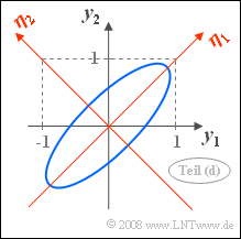
(4)  Correct are  the proposed solutions 1 and 2.

The eigenvectors are obtained by substituting the eigenvalues  $\lambda_1$  and  $\lambda_2$  into the correlation matrix:

$$\left[ \begin{array}{cc}1- (1+\rho) & \rho \\\rho & 1- (1+\rho)\end{array} \right]\cdot{\boldsymbol{\eta_1}} = \left[ \begin{array}{cc}-\rho & \rho \\\rho & -\rho\end{array} \right]\cdot \left[ \begin{array}{c}\eta_{11} \\\eta_{12}\end{array} \right]=0$$:$$\Rightarrow\hspace{0.3cm}-\rho \cdot \eta_{11} + \rho \cdot\eta_{12} = 0\hspace{0.3cm}\Rightarrow\hspace{0.3cm}\eta_{11}={\rm const} \cdot\eta_{12}\hspace{0.3cm}\Rightarrow\hspace{0.3cm}{\boldsymbol{\eta_1}}={\rm const}\cdot \left[ \begin{array}{c}1 \\1\end{array} \right];$$:$$\left[ \begin{array}{cc}1- (1-\rho) & \rho \\\rho & 1- (1-\rho)\end{array} \right]\cdot{\boldsymbol{\eta_2}} = \left[ \begin{array}{cc}\rho & \rho \\\rho & \rho\end{array} \right]\cdot \left[ \begin{array}{c}\eta_{21} \\\eta_{22}\end{array} \right]=0$$:$$\Rightarrow\hspace{0.3cm}\rho \cdot \eta_{21} + \rho \cdot\eta_{22} = 0\hspace{0.3cm}\Rightarrow\hspace{0.3cm}\eta_{21}=-{\rm const} \cdot\eta_{22}\hspace{0.3cm}\Rightarrow\hspace{0.3cm}{\boldsymbol{\eta_2}}={\rm const}\cdot \left[ \begin{array}{c}-1 \\1\end{array} \right].$$
Rotate the coordinate system
Putting this into the  "orthonormal form",  the following holds::$${\boldsymbol{\eta_1}}= \frac{1}{\sqrt{2}}\cdot \left[\begin{array}{c}1 \\1\end{array} \right],\hspace{0.5cm}{\boldsymbol{\eta_2}}= \frac{1}{\sqrt{2}}\cdot \left[\begin{array}{c}-1 \\1\end{array} \right].$$

The sketch illustrates the result:

  • The coordinate system defined by  $\mathbf{\eta_1}$  and  $\mathbf{\eta_2}$  is actually in the direction of the main axes of the original system.
  • With  $\sigma_1 = \sigma_2$  almost always results  $($exception:   $\rho= 0)$  the rotation angle  $\alpha = 45^\circ$.
  • This also follows from the equation given in the theory section:
$$\alpha = {1}/{2}\cdot \arctan (2 \cdot\rho \cdot\frac{\sigma_1\cdot\sigma_2}{\sigma_1^2 -\sigma_2^2})={1}/{2}\cdot \arctan(\infty)\hspace{0.3cm}\rightarrow\hspace{0.3cm}\alpha = 45^\circ.$$
  • The eigenvalues  $\lambda_1$  and  $\lambda_2$  do not denote the standard deviations with respect to the new axes, but the variances.


(5)  By comparing the matrices   $\mathbf{K_x}$   and   $\mathbf{K_z}$   we get.

  • $\sigma_{1}\hspace{0.15cm}\underline{ =2}$,
  • $\sigma_{2}\hspace{0.15cm}\underline{ =1}$,
  • $\rho = 2/(\sigma_{1} \cdot \sigma_{2})\hspace{0.15cm}\underline{ =1}$.


(6)  According to the now familiar scheme:

$$(4- \lambda) \cdot (1- \lambda) -4 = 0\hspace{0.3cm}\Rightarrow\hspace{0.3cm}\lambda^2 - 5\lambda =0\hspace{0.3cm}\Rightarrow\hspace{0.3cm}\hspace{0.15cm}\underline{\lambda_{1}=5,\hspace{0.1cm} \lambda_{2} =0}.$$


(7)  According to the equation given on the specification sheet:

$$\alpha ={1}/{2}\cdot \arctan (2 \cdot 1 \cdot \frac{2 \cdot1}{2^2 -1^2})= {1}/{2}\cdot \arctan ({4}/{3}) =26.56^\circ.$$
Best possible decorrelation

The same result is obtained using the eigenvector:

$$\left[ \begin{array}{cc}4-5 & 2 \\2 & 1-5\end{array} \right]\cdot \left[ \begin{array}{c}\zeta_{11} \\\zeta_{12}\end{array}\right]=0 \hspace{0.3cm}\Rightarrow\hspace{0.3cm}-\zeta_{11}=2\zeta_{12}=0\hspace{0.3cm}\Rightarrow\hspace{0.3cm}\zeta_{12}={\zeta_{11}}/{2}$$:$$\Rightarrow\hspace{0.3cm}\alpha = \arctan({\zeta_{12}}/{\zeta_{11}}) = \arctan(0.5) \hspace{0.15cm}\underline{= 26.56^\circ}.$$

The accompanying sketch shows the joint PDF of the random variable  $\mathbf{z}$:

  • Because of  $\rho = 1$  all values lie on the correlation line with coordinates  $z_1$  and  $z_2 = z_1/2$.
  • By rotating by the angle   $\alpha = \arctan(0.5) = 26.56^\circ$   a new coordinate system is formed.
  • The variance along the axis   $\mathbf{\zeta_1}$   is  $\lambda_1 = 5$  $($standard deviation  $\sigma_1 = \sqrt{5} = 2.236)$,
  • while in the direction orthogonal to it,  the random variable  $\mathbf{\zeta_2}$  is not extended  $(\lambda_2 = \sigma_2 = 0)$.