Difference between revisions of "Aufgaben:Exercise 1.3: Measured Step Response"
| Line 87: | Line 87: | ||
'''(3)''' The step response $σ(t)$ is equal to the output signal $y(t)$ if $x(t) = γ(t)$ is applied to the input. | '''(3)''' The step response $σ(t)$ is equal to the output signal $y(t)$ if $x(t) = γ(t)$ is applied to the input. | ||
| − | * | + | *Because of $x_1(t) = 4 \hspace{0.05cm} \rm {V} · γ(t)$ the following holds in the range from $0$ to $T = 2 \ \rm ms$: |
:$$\sigma(t) = \frac{y_1(t)}{ {\rm 4\, V} } = 0.5 \cdot\big( {t}/{T} - 0.5 ({t}/{T})^2\big).$$ | :$$\sigma(t) = \frac{y_1(t)}{ {\rm 4\, V} } = 0.5 \cdot\big( {t}/{T} - 0.5 ({t}/{T})^2\big).$$ | ||
| − | * | + | *At time $t = T = 2 \ \rm ms$ the step response reaches its final value $0.25$. |
| − | * | + | *For $t = T/2 = 1 \ \rm ms$ the numerical value $3/16 \; \underline{\: = \: 0.1875}$ is obtained. |
| − | * | + | *Please note that the step response $σ(t)$ as well as the step function $γ(t)$ has no unit. |
| − | [[File:P_ID840__LZI_A_1_3d.png | | + | [[File:P_ID840__LZI_A_1_3d.png |Computed impulse response | rechts|frame]] |
| − | '''(4)''' | + | '''(4)''' The step response $σ(t)$ is the integral over the impulse response $h(t)$. |
| − | * | + | *Thus, $h(t)$ is obtained from $σ(t)$ by differentiation with respect to time. |
| − | * | + | *n the range $0 < t < T$ therefore the following is valid: |
:$$h(t) = \frac{{\rm d}\hspace{0.1cm}\sigma(t)}{{\rm d}t}= 0.5 \cdot\left( \frac{1}{T} - 0.5 (\frac{2t}{T^2})\right) = \frac{0.5}{T} \cdot (1- \frac{t}{T})$$ | :$$h(t) = \frac{{\rm d}\hspace{0.1cm}\sigma(t)}{{\rm d}t}= 0.5 \cdot\left( \frac{1}{T} - 0.5 (\frac{2t}{T^2})\right) = \frac{0.5}{T} \cdot (1- \frac{t}{T})$$ | ||
:$$\Rightarrow \hspace{0.2cm} h(t = {\rm 1\, ms}) = h(t = T/2) = \frac{0.25}{T} \hspace{0.15cm}\underline{= 125 \cdot{1}/{ {\rm s} } },$$ | :$$\Rightarrow \hspace{0.2cm} h(t = {\rm 1\, ms}) = h(t = T/2) = \frac{0.25}{T} \hspace{0.15cm}\underline{= 125 \cdot{1}/{ {\rm s} } },$$ | ||
:$$\Rightarrow \hspace{0.2cm} h(t = {\rm 2\, ms}) = h(t = T) \hspace{0.15cm}\underline{= 0}.$$ | :$$\Rightarrow \hspace{0.2cm} h(t = {\rm 2\, ms}) = h(t = T) \hspace{0.15cm}\underline{= 0}.$$ | ||
| − | * | + | *For $t < 0$ and $t ≥ T$ this, $h(t)=0$, always holds. |
| − | * | + | *The value $h(t = 0)$ at exactly $t = 0$ must be determined from the mean value between the left-hand and right-hand limits: |
:$$h(t=0) = {1}/{2} \cdot \left[ \lim_{\varepsilon | :$$h(t=0) = {1}/{2} \cdot \left[ \lim_{\varepsilon | ||
\hspace{0.03cm} \to \hspace{0.03cm}0} h(- \varepsilon)+ \lim_{\varepsilon | \hspace{0.03cm} \to \hspace{0.03cm}0} h(- \varepsilon)+ \lim_{\varepsilon | ||
| Line 110: | Line 110: | ||
| − | [[File:P_ID829__LZI_A_1_3e.png | | + | [[File:P_ID829__LZI_A_1_3e.png | computed rectangular response| rechts|frame]] |
| − | '''(5)''' | + | '''(5)''' The rectangular pulse $x_2(t)$ can also be represented as the difference of two steps shifted by $±T/2$ : |
:$$x_2(t) = A \cdot \big[\gamma(t + {T}/{2}) - \gamma(t - {T}/{2})\big].$$ | :$$x_2(t) = A \cdot \big[\gamma(t + {T}/{2}) - \gamma(t - {T}/{2})\big].$$ | ||
| − | * | + | *Hence, the output signal is equal to the difference of two step responses shifted by $±T/2$ : |
:$$y_2(t) = A \cdot \big[\sigma(t + {T}/{2}) - \sigma(t - {T}/{2})\big].$$ | :$$y_2(t) = A \cdot \big[\sigma(t + {T}/{2}) - \sigma(t - {T}/{2})\big].$$ | ||
| − | * | + | *For $t = \: -T/2 = -1\ \rm ms$ the following holds: $y_2(t) \;\underline{ = 0}$. |
| − | * | + | *For the other time points considered the following is obtained as indicated in the graph: |
:$$y_2(t = 0) = A \cdot \big[\sigma(0.5 \cdot T) - \sigma(-0.5 \cdot T)\big] = | :$$y_2(t = 0) = A \cdot \big[\sigma(0.5 \cdot T) - \sigma(-0.5 \cdot T)\big] = | ||
{\rm 2\, V}\cdot \left[0.1875 - 0\right] \hspace{0.15cm}\underline{= {\rm 0.375\, V}},$$ | {\rm 2\, V}\cdot \left[0.1875 - 0\right] \hspace{0.15cm}\underline{= {\rm 0.375\, V}},$$ | ||
Revision as of 02:09, 1 July 2021
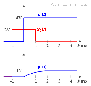
A step-shaped signal $$x_1(t) = 4\hspace{0.05cm} {\rm V} \cdot \gamma(t)$$ (blue curve) is applied to the input of a linear time-invariant (LTI) transmission system
- with the frequency response $H(f)$
- and the impulse response $h(t)$.
The measured output signal $y_1(t)$ then has the curve shown below.
- With $T = 2 \,{\rm ms}$ this signal can be described in the range from $0$ to $T$ as follows:
- $$y_1(t) = 2 \hspace{0.05cm}{\rm V} \cdot\big[ {t}/{T} - 0.5 \cdot ({t}/{T})^2\big].$$
- From $t = T $ on $y_1(t)$ is constantly equal $1 \,{\rm V}$.
In the last subtask (5) the output signal $y_2(t)$ is to be determined if a symmetrical rectangular pulse $x_2(t)$ of duration $T = 2 \hspace{0.05cm} {\rm ms}$ is applied to the input (see red curve in the upper graph).
Please note:
- The task belongs to the chapter System Description in Time Domain.
- The rectangular pulse $x_2(t)$ can also be written as follows with $A = 2 \hspace{0.05cm} \text{V}$ :
- $$x_2(t) = A \cdot \big [\gamma(t + {T}/{2}) - \gamma(t - {T}/{2})\big ].$$
- The frequency response $H(f)$ of the LTI system considered here can be taken from the exercise description of Exercise 3.8 in the book "Signal Representation”. However, the abscissa and ordinate parameters have to be adjusted accordingly.
- For the solution of the problem on hand, though, $H(f)$ is not explicitly required.
Questions
Sample solution
- The output signal is $y_1(t)=0$ as long as the input signal is $x_1(t) = 0$ . This means that there is a causal system on hand.
- One could have arrived at the same result just by considering the statement "the output signal was measured". Only causal systems are realisable and only in realisable systems something can be measured.
- The input signal $x_1(t)$ can be interpreted as a direct signal for very large times $(t \gg 0)$ . If $H(f)$ was a high-pass filter, then $y_1(t)$ would have to go towards zero for $t → ∞$ . This means: $H(f)$ represents a low-pass filter.
(2) The direct signal transmission factor can be read from $x_1(t)$ and $y_1(t)$ when the transient has decayed:
- $$H(f =0) = \frac{y_1(t \rightarrow \infty)}{x_1(t \rightarrow \infty)}= \frac{ {\rm 1\, V} }{ {\rm 4\, V} } \hspace{0.15cm}\underline{= 0.25}.$$
(3) The step response $σ(t)$ is equal to the output signal $y(t)$ if $x(t) = γ(t)$ is applied to the input.
- Because of $x_1(t) = 4 \hspace{0.05cm} \rm {V} · γ(t)$ the following holds in the range from $0$ to $T = 2 \ \rm ms$:
- $$\sigma(t) = \frac{y_1(t)}{ {\rm 4\, V} } = 0.5 \cdot\big( {t}/{T} - 0.5 ({t}/{T})^2\big).$$
- At time $t = T = 2 \ \rm ms$ the step response reaches its final value $0.25$.
- For $t = T/2 = 1 \ \rm ms$ the numerical value $3/16 \; \underline{\: = \: 0.1875}$ is obtained.
- Please note that the step response $σ(t)$ as well as the step function $γ(t)$ has no unit.
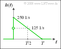
(4) The step response $σ(t)$ is the integral over the impulse response $h(t)$.
- Thus, $h(t)$ is obtained from $σ(t)$ by differentiation with respect to time.
- n the range $0 < t < T$ therefore the following is valid:
- $$h(t) = \frac{{\rm d}\hspace{0.1cm}\sigma(t)}{{\rm d}t}= 0.5 \cdot\left( \frac{1}{T} - 0.5 (\frac{2t}{T^2})\right) = \frac{0.5}{T} \cdot (1- \frac{t}{T})$$
- $$\Rightarrow \hspace{0.2cm} h(t = {\rm 1\, ms}) = h(t = T/2) = \frac{0.25}{T} \hspace{0.15cm}\underline{= 125 \cdot{1}/{ {\rm s} } },$$
- $$\Rightarrow \hspace{0.2cm} h(t = {\rm 2\, ms}) = h(t = T) \hspace{0.15cm}\underline{= 0}.$$
- For $t < 0$ and $t ≥ T$ this, $h(t)=0$, always holds.
- The value $h(t = 0)$ at exactly $t = 0$ must be determined from the mean value between the left-hand and right-hand limits:
- $$h(t=0) = {1}/{2} \cdot \left[ \lim_{\varepsilon \hspace{0.03cm} \to \hspace{0.03cm}0} h(- \varepsilon)+ \lim_{\varepsilon \hspace{0.03cm} \to \hspace{0.03cm} 0} h(+ \varepsilon)\right] = \left[ 0 + {0.5}/{T}\right] = {0.25}/{T}= 250 \cdot{1}/{ {\rm s} }.$$
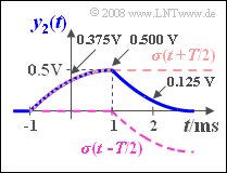
(5) The rectangular pulse $x_2(t)$ can also be represented as the difference of two steps shifted by $±T/2$ :
- $$x_2(t) = A \cdot \big[\gamma(t + {T}/{2}) - \gamma(t - {T}/{2})\big].$$
- Hence, the output signal is equal to the difference of two step responses shifted by $±T/2$ :
- $$y_2(t) = A \cdot \big[\sigma(t + {T}/{2}) - \sigma(t - {T}/{2})\big].$$
- For $t = \: -T/2 = -1\ \rm ms$ the following holds: $y_2(t) \;\underline{ = 0}$.
- For the other time points considered the following is obtained as indicated in the graph:
- $$y_2(t = 0) = A \cdot \big[\sigma(0.5 \cdot T) - \sigma(-0.5 \cdot T)\big] = {\rm 2\, V}\cdot \left[0.1875 - 0\right] \hspace{0.15cm}\underline{= {\rm 0.375\, V}},$$
- $$y_2(t = T/2) = y_2(t = 1\,{\rm ms}) =A \cdot \big[\sigma( T) - \sigma(0)\big] = {\rm 2\, V}\cdot \left[0.25 - 0\right] \hspace{0.15cm}\underline{= {\rm 0.5\, V}},$$
- $$y_2(t = T) = A \cdot \big[\sigma(1.5 \cdot T) - \sigma(0.5 \cdot T)\big] = {\rm 2\, V}\cdot \big[0.25 - 0.1875\big] \hspace{0.15cm}\underline{= {\rm 0.125\, V}}.$$


