Difference between revisions of "Aufgaben:Exercise 3.10Z: Rayleigh? Or Rice?"
From LNTwww
| Line 3: | Line 3: | ||
}} | }} | ||
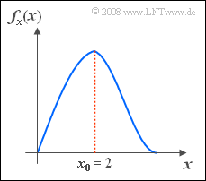
| − | [[File:P_ID149__Sto_Z_3_10.png|right|frame|Does the present PDF describe Rayleigh or Rice?]] | + | [[File:P_ID149__Sto_Z_3_10.png|right|frame|Does the present PDF describe "Rayleigh" or "Rice"?]] |
The probability density function of the random variable $x$ is given as follows: | The probability density function of the random variable $x$ is given as follows: | ||
:$$f_x(x)=\frac{\it x}{\lambda^{2}}\cdot{\rm e}^{-x^{\rm 2}/(\lambda^{\rm 2})}.$$ | :$$f_x(x)=\frac{\it x}{\lambda^{2}}\cdot{\rm e}^{-x^{\rm 2}/(\lambda^{\rm 2})}.$$ | ||
| − | Correspondingly, for the associated distribution function: | + | Correspondingly, for the associated distribution function: |
:$$F_x(r)= {\rm Pr}(x \le r) = 1-{\rm e}^{- r^{\rm 2}/(2 \lambda^{\rm 2})}.$$ | :$$F_x(r)= {\rm Pr}(x \le r) = 1-{\rm e}^{- r^{\rm 2}/(2 \lambda^{\rm 2})}.$$ | ||
*It is known that the value $x_0 = 2$ occurs most frequently. | *It is known that the value $x_0 = 2$ occurs most frequently. | ||
| − | *This also means that the PDF $f_x(x)$ is maximum at $x = x_0 $ | + | *This also means that the PDF $f_x(x)$ is maximum at $x = x_0 $. |
| − | |||
| − | |||
| − | |||
| Line 21: | Line 18: | ||
Hints: | Hints: | ||
This exercise belongs to the chapter [[Theory_of_Stochastic_Signals/Further_Distributions|Further Distributions]]. | This exercise belongs to the chapter [[Theory_of_Stochastic_Signals/Further_Distributions|Further Distributions]]. | ||
| − | *In particular, reference is made to the pages [[Theory_of_Stochastic_Signals/Further_Distributions#Rayleigh_PDF|Rayleigh PDF]] and [[Theory_of_Stochastic_Signals/Further_Distributions#Rice_PDF|Rice PDF]] . | + | *In particular, reference is made to the pages [[Theory_of_Stochastic_Signals/Further_Distributions#Rayleigh_PDF|Rayleigh PDF]] and [[Theory_of_Stochastic_Signals/Further_Distributions#Rice_PDF|Rice PDF]] . |
| − | + | *You can check your results with interactive applet [[Applets:WDF,_VTF_und_Momente_spezieller_Verteilungen_(Applet)|PDF, CDF and moments of special distributions]]. | |
| − | *You can check your results with interactive applet [[Applets:WDF,_VTF_und_Momente_spezieller_Verteilungen_(Applet)|PDF, CDF and moments of special distributions]] . | + | *You can check your results with interactive applet [[Applets:PDF,_CDF_and_Moments_of_Special_Distributions|PDF, CDF and moments of special distributions]]. |
*Consider the following definite integral in the solution: | *Consider the following definite integral in the solution: | ||
:$$\int_{0}^{\infty}x^{\rm 2}\cdot {\rm e}^{ -x^{\rm 2}/\rm 2} \, {\rm d}x=\sqrt{{\pi}/{\rm 2}}.$$ | :$$\int_{0}^{\infty}x^{\rm 2}\cdot {\rm e}^{ -x^{\rm 2}/\rm 2} \, {\rm d}x=\sqrt{{\pi}/{\rm 2}}.$$ | ||
Revision as of 11:32, 3 February 2022
The probability density function of the random variable $x$ is given as follows:
- $$f_x(x)=\frac{\it x}{\lambda^{2}}\cdot{\rm e}^{-x^{\rm 2}/(\lambda^{\rm 2})}.$$
Correspondingly, for the associated distribution function:
- $$F_x(r)= {\rm Pr}(x \le r) = 1-{\rm e}^{- r^{\rm 2}/(2 \lambda^{\rm 2})}.$$
- It is known that the value $x_0 = 2$ occurs most frequently.
- This also means that the PDF $f_x(x)$ is maximum at $x = x_0 $.
Hints:
This exercise belongs to the chapter Further Distributions.
- In particular, reference is made to the pages Rayleigh PDF and Rice PDF .
- You can check your results with interactive applet PDF, CDF and moments of special distributions.
- You can check your results with interactive applet PDF, CDF and moments of special distributions.
- Consider the following definite integral in the solution:
- $$\int_{0}^{\infty}x^{\rm 2}\cdot {\rm e}^{ -x^{\rm 2}/\rm 2} \, {\rm d}x=\sqrt{{\pi}/{\rm 2}}.$$
Questions
Solution
(1) Correct is only the second proposed solution.
- Because of the given PDF there is no Rice distribution, but a Rayleigh distribution.
- This is asymmetric around the mean $m_x$ so that $\mu_3 \ne 0$ .
- Only in the case of a smoothly distributed random size does the kurtosis $K = 3$.
- For the Rayleigh distribution, a larger value $(K = 3.245)$ is obtained due to more pronounced PDF–emitters, independent of $\lambda$.
(2) The derivative of the PDF with respect to $x$ yields:
- $$\frac{{\rm d} f_x(x)}{{\rm d} x} = \frac{\rm 1}{\lambda^{\rm 2}}\cdot{\rm e}^{ -{x^{\rm 2}}/({2 \lambda^{\rm 2}})}+\frac{ x}{ \lambda^{\rm 2}}\cdot{\rm e}^{ -{x^{\rm 2}}/({ 2 \lambda^{\rm 2}})}\cdot(-\frac{2 x}{2 \lambda^{\rm 2}}).$$
- From this follows as the equation of determination for $x_0$ (only the positive solution is meaningful):
- $$\frac{1}{\lambda^{\rm 2}}\cdot{\rm e}^{ -{x_{\rm 0}^{\rm 2}}/{(2 \lambda^{\rm 2}})}\cdot(\rm 1-{\it x_{\rm 0}^{\rm 2}}/{\it \lambda^{\rm 2}})=0 \quad \Rightarrow \quad {\it x}_0=\it \lambda.$$
- Thus, we obtain for the distribution parameter $\lambda = x_0\hspace{0.15cm}\underline{= 2}$.
(3) The probability we are looking for is equal to the distribution function at the point $r = x_0 = \lambda$:
- $${\rm Pr}(x<x_{\rm 0})={\rm Pr}( x \le x_{\rm 0})= F_x(x_{\rm 0})=1-{\rm e}^{-{\lambda^{\rm 2}}/({ 2 \lambda^{\rm 2}})}=1-{\rm e}^{-0.5}\hspace{0.15cm}\underline{=\rm 39.3\%}.$$
(4) For example, the mean can be calculated using the following equation:
- $$m_x=\int_{-\infty}^{+\infty}\hspace{-0.45cm}x\cdot f_x(x)\,{\rm d}x=\int_{\rm 0}^{\infty}\frac{\it x^{\rm 2}}{\it \lambda^{\rm 2}} \cdot \rm e^{-{\it x^{\rm 2}}/({\rm 2\it \lambda^{\rm 2}})}\,{\rm d}\it x = \sqrt{{\rm \pi}/{\rm 2}}\cdot \it \lambda\hspace{0.15cm}\underline{=\rm 2.506}.$$
- The mean $m_x$ is of course larger than $x_0$ $(=$ maximum value of the PDF$)$, since the PDF is bounded downward but not upward.
(5) In general, for the sought probability:
- $${\rm Pr}(x>m_x)=1- F_x(m_x).$$
- With the given distribution function and the result of the subtask (4) we obtain:
- $${\rm Pr}(x>m_x)={\rm e}^{-{m_x^{\rm 2}}/({ 2\lambda^{\rm 2})}}={\rm e}^{-\pi/ 4}\hspace{0.15cm}\underline{\approx \rm 45.6\%}.$$
