Difference between revisions of "Aufgaben:Exercise 4.8Z: AWGN Channel"
From LNTwww
| Line 3: | Line 3: | ||
}} | }} | ||
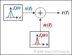
| − | [[File:P_ID413__Sto_Z_4_8.png|right|frame| | + | [[File:P_ID413__Sto_Z_4_8.png|right|frame|Channel model "AWGN"]] |
| − | We consider here an analog message signal $s(t)$ whose amplitude values are Gaussian distributed. | + | We consider here an analog message signal $s(t)$ whose amplitude values are Gaussian distributed. The standard deviation of this zero mean signal is $\sigma_s=1 \hspace{0.05cm} \rm V$. |
| − | |||
| − | |||
| − | + | During transmission $s(t)$ is additively overlaid by noise $n(t)$ which like $s(t)$ can be assumed to be Gaussian distributed and zero mean. | |
| − | + | *Let the standard deviation of the noise be generally $\sigma_n$. | |
| − | During transmission $s(t)$ is additively overlaid by | + | *It is assumed that there are no statistical dependencies between the signals $s(t)$ and $n(t)$. |
| − | *Let the | + | *Such a constellation is called "Additive White Gaussian Noise" $\rm (AWGN)$. |
| − | *It is assumed that there are no statistical dependencies between | + | *The quality criterion for the received signal $r(t)= s(t)+n(t)$ the "signal-to-noise power ratio": |
| − | |||
| − | |||
| − | Such a constellation is called | ||
:$${\rm SNR} = {\sigma_s^2}/{\sigma_n^2}.$$ | :$${\rm SNR} = {\sigma_s^2}/{\sigma_n^2}.$$ | ||
| Line 21: | Line 16: | ||
| − | + | Hints: | |
| − | |||
| − | |||
*The exercise belongs to the chapter [[Theory_of_Stochastic_Signals/Linear_Combinations_of_Random_Variables|Linear Combinations of Random Variables]]. | *The exercise belongs to the chapter [[Theory_of_Stochastic_Signals/Linear_Combinations_of_Random_Variables|Linear Combinations of Random Variables]]. | ||
*Reference is also made to the chapter [[Theory_of_Stochastic_Signals/Two-Dimensional_Gaussian_Random_Variables|Two-dimensional Gaussian random variables]]. | *Reference is also made to the chapter [[Theory_of_Stochastic_Signals/Two-Dimensional_Gaussian_Random_Variables|Two-dimensional Gaussian random variables]]. | ||
| Line 33: | Line 26: | ||
<quiz display=simple> | <quiz display=simple> | ||
| − | {Give the PDF $f_r(r)$ of the received signal $r(t)$ in general. What is the | + | {Give the PDF $f_r(r)$ of the received signal $r(t)$ in general. What is the standard deviation $\sigma_r$ when $\sigma_n =0.75 \hspace{0.05cm} \rm V$? |
|type="{}"} | |type="{}"} | ||
$\sigma_r \ = \ $ { 1.25 3% } $ \ \rm V$ | $\sigma_r \ = \ $ { 1.25 3% } $ \ \rm V$ | ||
| Line 43: | Line 36: | ||
| − | {Calculate the correlation coefficient $\rho_{sr}$ depending on the SNR of the AWGN channel. Derive an approximation for large SNR. | + | {Calculate the correlation coefficient $\rho_{sr}$ depending on the SNR of the AWGN channel. Derive an approximation for large SNR. |
| + | |type="{}"} | ||
| + | $\rho_{sr} \ = \ $ { 0.8 3% } | ||
Latest revision as of 16:22, 27 February 2022
We consider here an analog message signal $s(t)$ whose amplitude values are Gaussian distributed. The standard deviation of this zero mean signal is $\sigma_s=1 \hspace{0.05cm} \rm V$.
During transmission $s(t)$ is additively overlaid by noise $n(t)$ which like $s(t)$ can be assumed to be Gaussian distributed and zero mean.
- Let the standard deviation of the noise be generally $\sigma_n$.
- It is assumed that there are no statistical dependencies between the signals $s(t)$ and $n(t)$.
- Such a constellation is called "Additive White Gaussian Noise" $\rm (AWGN)$.
- The quality criterion for the received signal $r(t)= s(t)+n(t)$ the "signal-to-noise power ratio":
- $${\rm SNR} = {\sigma_s^2}/{\sigma_n^2}.$$
Hints:
- The exercise belongs to the chapter Linear Combinations of Random Variables.
- Reference is also made to the chapter Two-dimensional Gaussian random variables.
Questions
Solution
(1) It holds $r(t) = s(t)+n(t)$. Thus $f_r(r)$ can be calculated from the convolution of the two density functions $f_s(s)$ and $f_n(n)$ .
- Since both signals are Gaussian distributed, the convolution also yields a Gaussian function:
$$f_r(r)= \frac {1}{\sqrt{2 \pi} \cdot \sigma_r} \cdot {\rm e}^{-r^2/(2 \sigma_r^2)}.$$
- The variances of $s(t)$ and $n(t)$ add up. Therefore, with $\sigma_s =1 \hspace{0.05cm} \rm V$ and $\sigma_n =0.75 \hspace{0.05cm} \rm V$:
- $$\sigma_r = \sqrt{\sigma_s^2 + \sigma_n^2} =\sqrt{{(\rm 1\hspace{0.1cm}V)^2} + {(\rm 0.75\hspace{0.1cm}V)^2}}\hspace{0.15cm}\underline{ = {\rm 1.25\hspace{0.1cm}V}}.$$
(2) For the correlation coefficient, with the joint moment $m_{sr}$:
- $$\rho_{sr } = \frac{m_{sr }}{\sigma_s \cdot \sigma_r}.$$
- This takes into account that $s(t)$ and also $r(t)$ are zero mean, so that $\mu_{sr} =m_{sr}$ holds.
- Since $s(t)$ and $n(t)$ were assumed to be statistically independent of each other and thus uncorrelated, it further holds:
- $$m_{sr} = {\rm E}\big[s(t) \cdot r(t)\big] = {\rm E}\big[s^2(t)\big] + {\rm E}\big[s(t) \cdot n(t)\big] ={\rm E}\big[s^2(t)\big] = \sigma_s^2.$$
- $$\rightarrow \hspace{0.3cm} \rho_{sr } = \frac{\sigma_s}{ \sigma_r} = \sqrt{\frac{\sigma_s^2}{\sigma_s^2 + \sigma_n^2}} = \left (1+ {\sigma_n^2}/{\sigma_s^2}\right)^{-1/2}.$$
- With $\sigma_s =1 \hspace{0.05cm} \rm V$, $\sigma_n =0.75 \hspace{0.05cm} \rm V$ and $\sigma_r =1.25 \hspace{0.05cm} \rm V$ one obtains $\rho_{sr }\hspace{0.15cm}\underline{ = 0.8}$.
(3) The expression calculated in the last subtask can be represented by the abbreviation ${\rm SNR} =\sigma_s^2/\sigma_n^2$ as follows:
- $$\rho_{sr } = \rm \frac{1}{ \sqrt{1 + \frac{1}{SNR}}} \approx \frac{1}{ {1 + \frac{1}{2 \cdot SNR}}} \approx 1 - \frac{1}{2 \cdot SNR}.$$
- The signal-to-noise ratio $10 \cdot {\rm lg \ SNR = 30 \ dB}$ leads to the absolute value $\rm SNR = 1000$.
- Inserted into the above equation, this gives an approximate correlation coefficient of $\rho_{sr }\hspace{0.15cm}\underline{ = 0.9995}$.
