Difference between revisions of "Aufgaben:Exercise 4.10Z: Correlation Duration"
| Line 3: | Line 3: | ||
}} | }} | ||
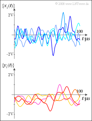
| − | [[File:P_ID393__Sto_Z_4_10.png|right|frame| | + | [[File:P_ID393__Sto_Z_4_10.png|right|frame|Pattern signals of ergodic processes]] |
The graphic shows pattern signals of two random processes $\{x_i(t)\}$ and $\{y_i(t)\}$ with equal power | The graphic shows pattern signals of two random processes $\{x_i(t)\}$ and $\{y_i(t)\}$ with equal power | ||
:$$P_x = P_y = 5\hspace{0.05 cm} \rm mW.$$ | :$$P_x = P_y = 5\hspace{0.05 cm} \rm mW.$$ | ||
Revision as of 19:40, 20 March 2022
The graphic shows pattern signals of two random processes $\{x_i(t)\}$ and $\{y_i(t)\}$ with equal power
- $$P_x = P_y = 5\hspace{0.05 cm} \rm mW.$$
Assuming here the resistance $R = 50\hspace{0.05 cm}\rm \Omega$.
The random process $\{x_i(t)\}$
- is zero mean $(m_x = 0)$,
- has the Gaussian ACF $\varphi_x (\tau) = \varphi_x (\tau = 0) \cdot {\rm e}^{- \pi \hspace{0.03cm} \cdot \hspace{0.03cm}(\tau / {\rm \nabla} \tau_x)^2},$ and
- exhibits the equivalent ACF duration $\nabla \tau_x = 5\hspace{0.05 cm}\rm µ s $ .
As can be seen from the diagram below, the random process $\{y_i(t)\}$ has much stronger internal statistical bindings than the random process $\{x_i(t)\}$.
Or, to put it another way:
- The random process $\{y_i(t)\}$ is lower frequency than $\{x_i(t)\}$.
- The equivalent ACF duration is $\nabla \tau_y = 10 \hspace{0.05 cm}\rm µ s $.
From the sketch it can also be seen that $\{y_i(t)\}$ in contrast to $\{x_i(t)\}$ is not DC free. The DC signal component is rather $m_y = -0.3 \hspace{0.05 cm}\rm V$.
Hint:
- The exercise belongs to the chapter Auto-Correlation Function.
- Reference is made in particular to the section Interpretation of the auto-correlation function.
Questions
Solution
- From this follows the standard deviation $\sigma_x\hspace{0.15 cm}\underline{= 0.5\hspace{0.05 cm}{\rm V}}$.
(2) Because $P_x = \varphi_x (\tau = 0)$ holds for the ACF in general:
- $$\varphi_x (\tau) = 5 \hspace{0.1cm} {\rm mW} \cdot {\rm e}^{- \pi \hspace{0.03cm} \cdot \hspace{0.03cm}(\tau / {\rm \nabla} \tau_x)^2}.$$
- From this we obtain:
- $$\varphi_x (\tau = {\rm 2\hspace{0.1cm} µ s}) = 5 \hspace{0.1cm} {\rm mW} \cdot {\rm e}^{- {\rm 0.16 }\pi } \hspace{0.15cm}\underline{= 3.025 \hspace{0.1cm} \rm mW},$$
- $$\varphi_x (\tau = {\rm 5\hspace{0.1cm} \rm µ s}) = 5 \hspace{0.1cm} {\rm mW} \cdot {\rm e}^{- \pi } \hspace{0.15cm}\underline{= 0.216 \hspace{0.1cm} \rm mW}.$$
(3) Here the following determination equation holds:
- $${\rm e}^{- \pi \hspace{0.03cm} \cdot \hspace{0.03cm}(T_{\rm K} / {\rm \nabla} \tau_x)^2} \stackrel{!}{=} {\rm 0.5} \hspace{0.5cm}\Rightarrow\hspace{0.5cm} (T_{\rm K} / {\rm \nabla} \tau_x)^2 = \sqrt{{ \ln(2)}/{\pi}}\hspace{0.05cm}.$$
- From this follows $T_{\rm K}\hspace{0.15 cm}\underline{= 2.35\hspace{0.05 cm}{\rm µ s}}$.
- With other ACF form, a different ratio is obtained for $T_{\rm K} / {\rm \nabla} \tau_x$.
(4) Because $P_x = P_y$ the root mean square values of $x$ and $y$ are equal, respectively $0.25\hspace{0.05 cm}\rm V^2$.
- Taking into account the mean value $m_y = -0.3 \hspace{0.05 cm}\rm V$ holds:
- $$m_y^2 + \sigma_y^2 = \rm 0.25 \hspace{0.05 cm} V^2.$$
- From this follows:
- $$\sigma_y\hspace{0.15 cm}\underline{= 0.4\hspace{0.05 cm}{\rm V}}.$$
(5) In terms of unit resistance $ R = 1 \hspace{0.05 cm}{\rm \Omega}$ the ASF of the process $\{y_i(t)\}$ is:
- $$\varphi_y (\tau) = m_y^2 + \sigma_y^2 \cdot {\rm e}^{- \pi \hspace{0.03cm} \cdot \hspace{0.03cm}(\tau / {\rm \nabla} \tau_y)^2}.$$
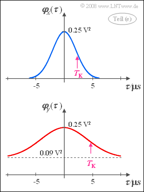
- On the right you can see the function progression. Related to the resistor $ R = 50 \hspace{0.05 cm}{\rm \Omega}$ results in the following ACF values:
- $$\varphi_y (\tau = 0) = 5 \hspace{0.1cm} {\rm mW} , \hspace{0.5cm} \varphi_y (\tau \rightarrow \infty) = 1.8\hspace{0.1cm} {\rm mW} .$$
- From this follows:
- $$\varphi_y(\tau) = 1.8 \hspace{0.1cm} {\rm mW} + 3.2 \hspace{0.1cm} {\rm mW} \cdot {\rm e}^{- \pi \hspace{0.03cm} \cdot \hspace{0.03cm}(\tau / {\rm \nabla} \tau_y)^2} \hspace{0.3cm }\Rightarrow \hspace{0.3cm }\varphi_y(\tau = 10\hspace{0.05 cm}{\rm µ s}) \hspace{0.15 cm}\underline{=1.938\hspace{0.05 cm}\rm mW}.$$
- With positive mean $m_y$ (having the same amplitude), there would be no change in the ASF, since $m_y$ is squared in the ASF equation.

