Difference between revisions of "Aufgaben:Exercise 4.2Z: About the Sampling Theorem"
| Line 71: | Line 71: | ||
===Solution=== | ===Solution=== | ||
{{ML-Kopf}} | {{ML-Kopf}} | ||
| − | '''(1)''' <u>All statements</u> are true: | + | '''(1)''' <u>All statements</u> are true: |
| − | [[File:P_ID1611__Mod_Z_4_2a.png|P_ID1611__Mod_Z_4_2a.png|right|frame|Spectral function of sampled signal]] | + | [[File:P_ID1611__Mod_Z_4_2a.png|P_ID1611__Mod_Z_4_2a.png|right|frame|Spectral function of the sampled signal]] |
| − | *The sampling theorem is satisfied by $f_{\rm A} = 11 \ \rm kHz > 2 \cdot 5 \ \rm kHz$ so that complete signal reconstruction is always possible. | + | *The sampling theorem is satisfied by $f_{\rm A} = 11 \ \rm kHz > 2 \cdot 5 \ \rm kHz$ so that a complete signal reconstruction is always possible. |
| − | *The spectrum $Q_{\rm A}(f)$ results from $Q(f)$ by periodic continuation at the respective frequency spacing $f_{\rm A}$, which is generally illustrated in the graph | + | *The spectrum $Q_{\rm A}(f)$ results from $Q(f)$ by periodic continuation at the respective frequency spacing $f_{\rm A}$, which is generally illustrated in the graph. |
| − | *By a | + | *By a rectangular low-pass with $f_{\rm G} = f_{\rm A}/2 = 5.5 \ \rm kHz$ the original spectrum $Q(f)$ is obtained. |
The shift by | The shift by | ||
| − | * $f_{\rm A} = 11 \ \rm kHz$ yields the lines at $+6 \ \rm kHz$ and $+16 \ \rm kHz$, | + | * $f_{\rm A} = 11 \ \rm kHz$ yields the lines at $+6 \ \rm kHz$ and $+16 \ \rm kHz$, |
| − | * $-f_{\rm A} = -11 \ \rm kHz$ yields the lines at $-6 \ \rm kHz$ and $-16 \ \rm kHz$, | + | * $-f_{\rm A} = -11 \ \rm kHz$ yields the lines at $-6 \ \rm kHz$ and $-16 \ \rm kHz$, |
| − | * $2 - f_{\rm A} = 22 \ \rm kHz$ yields the lines at $+17 \ \rm kHz$ and $+27 \ \rm kHz$, | + | * $2 - f_{\rm A} = 22 \ \rm kHz$ yields the lines at $+17 \ \rm kHz$ and $+27 \ \rm kHz$, |
* $-2 - f_{\rm A}= -22 \ \rm kHz$ yields the lines at $-17 \ \rm kHz$, $-27 \ \rm kHz$. | * $-2 - f_{\rm A}= -22 \ \rm kHz$ yields the lines at $-17 \ \rm kHz$, $-27 \ \rm kHz$. | ||
| Line 91: | Line 91: | ||
| − | '''(3)''' The correct solution is <u>suggestion 2</u>: | + | '''(3)''' The correct solution is <u>suggestion 2</u>: |
| − | *For the cosinusoidal signal, according to | + | [[File:P_ID1612__Mod_Z_4_2c.png|P_ID1612__Mod_Z_4_2c.png|right|frame|Spectral function of the sampled cosine signal]] |
| − | *The periodization of $Q(f)$ with $f_{\rm A} = 10 \rm kHz$ leads to a Dirac comb with spectral lines at $±f_{\rm N}$, $±f_{\rm N}± f_{\rm A}$, $±f_{\rm N}± 2f_{\rm A}$, . .. | + | |
| − | *Through the superpositions, all Dirac functions have weight $A$, while the | + | *For the cosinusoidal signal, according to this graph with $f_{\rm A} = 10 \rm \ kHz$: All spectral lines of $Q_{\rm A}(f)$: are real. |
| − | *Because $H(f = f_{\rm N}) = H(f = f_{\rm G}) = 0.5$ the spectrum $V_1(f)$ after the low-pass is identical to $Q_1(f)$ | + | *The periodization of $Q(f)$ with $f_{\rm A} = 10 \rm \ kHz$ leads to a Dirac comb with spectral lines at $±f_{\rm N}$, $±f_{\rm N}± f_{\rm A}$, $±f_{\rm N}± 2f_{\rm A}$, . .. |
| + | *Through the superpositions, all Dirac functions have weight $A$, while the spectral lines of $Q(f)$ are weighted only by $A/2$ each. | ||
| + | *Because $H(f = f_{\rm N}) = H(f = f_{\rm G}) = 0.5$ the spectrum $V_1(f)$ after the low-pass is identical to $Q_1(f)$ ⇒ $v_1(t) = q_1(t)$. | ||
*In the time domain, the signal reconstruction can be thought of as follows: The samples of $q_1(t)$ lie exactly at the signal maxima and minima. | *In the time domain, the signal reconstruction can be thought of as follows: The samples of $q_1(t)$ lie exactly at the signal maxima and minima. | ||
*The lowpass filter forms the cosine signal with correct amplitude, frequency and phase. | *The lowpass filter forms the cosine signal with correct amplitude, frequency and phase. | ||
| − | + | <br clear=all> | |
| − | + | [[File:P_ID1613__Mod_Z_4_2d.png|P_ID1613__Mod_Z_4_2d.png|right|frame|Sampled sine signal]] | |
| − | + | '''(4)''' Correct is <u>suggested solution 2</u>: | |
| − | + | *All sampled values of $q_2(t)$ now lie exactly at the zero crossings of the sinusoidal signal, which means that here $q_{\rm A}(t) \equiv 0$ holds. However, this naturally also gives $v_2(t) \equiv 0$. | |
| − | + | *In the spectral domain, the result can be derived using the graph for subtask '''(1)'''. <br>⇒ $Q(f)$ is purely imaginary and the imaginary parts at $±f_{\rm N}$ have different signs. | |
| − | [[File:P_ID1613__Mod_Z_4_2d.png|P_ID1613__Mod_Z_4_2d.png|right|frame| | + | *Thus, one positive and one negative part cancel each other in periodization <br>⇒ $Q_{\rm A}(f) \equiv 0$ ⇒ $V_2(f) \equiv 0$. |
| − | '''(4)''' Correct is <u>suggested solution 2</u>: | ||
| − | *All sampled values of $q_2(t)$ now lie exactly at the zero crossings of the sinusoidal signal, which means that here $q_{\rm A}(t) \equiv 0$ holds. However, this naturally also gives $v_2(t) \equiv 0$. | ||
| − | *In the spectral domain, the result can be derived using the graph for subtask '''(1)''' | ||
| − | *Thus, one positive and one negative part cancel each other in periodization ⇒ $Q_{\rm A}(f) \equiv 0$ ⇒ $V_2(f) \equiv 0$. | ||
<br clear=all> | <br clear=all> | ||
[[File:P_ID1614__Mod_Z_4_2e.png|P_ID1614__Mod_Z_4_2e.png|right|frame|Sampled harmonic oscillation with phase $φ_3 = π/4$]] | [[File:P_ID1614__Mod_Z_4_2e.png|P_ID1614__Mod_Z_4_2e.png|right|frame|Sampled harmonic oscillation with phase $φ_3 = π/4$]] | ||
| − | '''(5)''' <u>None of the given solutions</u> is correct: | + | '''(5)''' <u>None of the given solutions</u> is correct: |
| − | *If in the graph for the subtask '''(1)''' the sampling frequency $f_{\rm A} = 11 \ \rm kHz$ is replaced by $f_{\rm A} = 10 \ \rm kHz$, the real parts add up, but the imaginary parts cancel out. | + | *If in the graph for the subtask '''(1)''' the sampling frequency $f_{\rm A} = 11 \ \rm kHz$ is replaced by $f_{\rm A} = 10 \ \rm kHz$, the real parts add up, but the imaginary parts cancel out. |
| − | *This means that now $Q_{\rm A}(f)$ and $V_3(f)$ are real spectra. This further means | + | *This means that now $Q_{\rm A}(f)$ and $V_3(f)$ are real spectra. This further means: |
*The phase information is lost $(φ = 0)$ and the output signal $v_3(t)$ is a cosine signal. | *The phase information is lost $(φ = 0)$ and the output signal $v_3(t)$ is a cosine signal. | ||
| − | * | + | *$q_3(t)$ and $v_3(t)$ thus differ in both amplitude and phase. Only the frequency remains the same. |
The graph shows | The graph shows | ||
| − | *turquoise the signal $q_3(t)$ and its samples (circles) and | + | *turquoise the signal $q_3(t)$ and its samples (circles), and |
*red dashed the output signal $v_3(t)$ of the low-pass. | *red dashed the output signal $v_3(t)$ of the low-pass. | ||
| − | You can see that the | + | You can see that the low-pass gives exactly the result you would probably choose if you were to draw a curve through the samples (circles). |
Latest revision as of 12:28, 8 April 2022
The sampling theorem states that the sampling frequency $f_{\rm A} = 1/T_{\rm A}$ must be at least twice as large as the largest frequency $f_\text {N, max}$ contained in the source signal $q(t)$:
- $$f_{\rm A} \ge 2 \cdot f_{\rm N,\hspace{0.05cm}max}\hspace{0.3cm}\Rightarrow \hspace{0.3cm} T_{\rm A} \le \frac{1}{2 \cdot f_{\rm N, \hspace{0.05cm}max}}\hspace{0.05cm}.$$
If this condition is met, then at the receiver the message signal can be passed through a rectangular (ideal) low-pass filter with frequency response
- $$H(f) = \left\{ \begin{array}{l} 1 \\ 1/2 \\ 0 \\ \end{array} \right.\quad \begin{array}{*{5}c}{\rm{f\ddot{u}r}} \\{\rm{f\ddot{u}r}} \\{\rm{f\ddot{u}r}} \\ \end{array}\begin{array}{*{10}c} {\hspace{0.04cm}\left| \hspace{0.005cm} f\hspace{0.05cm} \right| < f_{\rm G},} \\ {\hspace{0.04cm}\left| \hspace{0.005cm} f\hspace{0.05cm} \right| = f_{\rm G},} \\ {\hspace{0.04cm}\left| \hspace{0.005cm} f\hspace{0.05cm} \right| > f_{\rm G}} \\ \end{array}$$
can be completely reconstructed, that is, it is then $v(t) = q(t)$.
- The cutoff frequency $f_{\rm G}$ is to be chosen equal to half the sampling frequency.
- The equal sign is generally valid only if the spectrum $Q(f)$ does not contain a discrete spectral line at frequency $f_\text {N, max}$.
In this exercise, three different source signals are considered, each of which can be expressed as a harmonic oscillation
- $$q(t) = A \cdot \cos (2 \pi \cdot f_{\rm N} \cdot t - \varphi)$$
with amplitude $A = 1\ \rm V$ and frequency $f_{\rm N}= 5 \ \rm kHz$. For the spectral function $Q(f)$ of all represented time signals generally holds:
- $$Q(f) = \frac{A}{2} \cdot \delta (f- f_{\rm N}) \cdot {\rm e}^{-{\rm j}\hspace{0.04cm}\cdot \hspace{0.04cm}\varphi}+ \frac{A}{2} \cdot \delta (f+ f_{\rm N}) \cdot {\rm e}^{+{\rm j}\hspace{0.04cm}\cdot \hspace{0.04cm}\varphi}\hspace{0.05cm}.$$
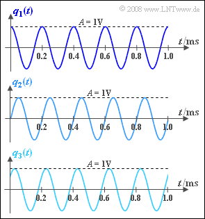
The oscillations sketched in the graph differ only by the phase $φ$:
- $φ_1 = 0$ ⇒ cosine signal $q_1(t)$,
- $φ_2 = π/2 \ (= 90^\circ)$ ⇒ sinusoidal signal $q_2(t)$,
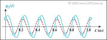
- $φ_3 = π/4 \ (= 45^\circ)$ ⇒ signal $q_3(t)$.
Hints:
- The exercise belongs to the chapter "Pulse Code Modulation".
- Reference is made in particular to the page "Sampling and Signal Reconstruction".
- The sampled source signal is denoted by $q_{\rm A}(t)$ and its spectral function by $Q_{\rm A}(f)$.
- Sampling is always performed at $ν \cdot T_{\rm A}$.
Questions
Solution
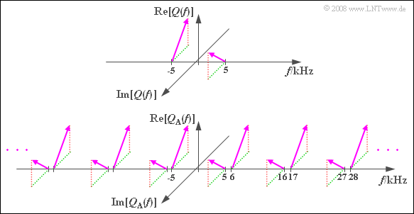
- The sampling theorem is satisfied by $f_{\rm A} = 11 \ \rm kHz > 2 \cdot 5 \ \rm kHz$ so that a complete signal reconstruction is always possible.
- The spectrum $Q_{\rm A}(f)$ results from $Q(f)$ by periodic continuation at the respective frequency spacing $f_{\rm A}$, which is generally illustrated in the graph.
- By a rectangular low-pass with $f_{\rm G} = f_{\rm A}/2 = 5.5 \ \rm kHz$ the original spectrum $Q(f)$ is obtained.
The shift by
- $f_{\rm A} = 11 \ \rm kHz$ yields the lines at $+6 \ \rm kHz$ and $+16 \ \rm kHz$,
- $-f_{\rm A} = -11 \ \rm kHz$ yields the lines at $-6 \ \rm kHz$ and $-16 \ \rm kHz$,
- $2 - f_{\rm A} = 22 \ \rm kHz$ yields the lines at $+17 \ \rm kHz$ and $+27 \ \rm kHz$,
- $-2 - f_{\rm A}= -22 \ \rm kHz$ yields the lines at $-17 \ \rm kHz$, $-27 \ \rm kHz$.
(2) The sampling distance is equal to the reciprocal of the sampling frequency:
- $$ T_{\rm A} = {1}/{f_{\rm A} }\hspace{0.15cm}\underline { = 0.1\,{\rm ms}} \hspace{0.05cm}.$$
(3) The correct solution is suggestion 2:
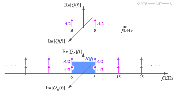
- For the cosinusoidal signal, according to this graph with $f_{\rm A} = 10 \rm \ kHz$: All spectral lines of $Q_{\rm A}(f)$: are real.
- The periodization of $Q(f)$ with $f_{\rm A} = 10 \rm \ kHz$ leads to a Dirac comb with spectral lines at $±f_{\rm N}$, $±f_{\rm N}± f_{\rm A}$, $±f_{\rm N}± 2f_{\rm A}$, . ..
- Through the superpositions, all Dirac functions have weight $A$, while the spectral lines of $Q(f)$ are weighted only by $A/2$ each.
- Because $H(f = f_{\rm N}) = H(f = f_{\rm G}) = 0.5$ the spectrum $V_1(f)$ after the low-pass is identical to $Q_1(f)$ ⇒ $v_1(t) = q_1(t)$.
- In the time domain, the signal reconstruction can be thought of as follows: The samples of $q_1(t)$ lie exactly at the signal maxima and minima.
- The lowpass filter forms the cosine signal with correct amplitude, frequency and phase.
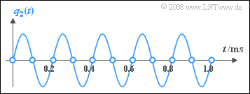
(4) Correct is suggested solution 2:
- All sampled values of $q_2(t)$ now lie exactly at the zero crossings of the sinusoidal signal, which means that here $q_{\rm A}(t) \equiv 0$ holds. However, this naturally also gives $v_2(t) \equiv 0$.
- In the spectral domain, the result can be derived using the graph for subtask (1).
⇒ $Q(f)$ is purely imaginary and the imaginary parts at $±f_{\rm N}$ have different signs. - Thus, one positive and one negative part cancel each other in periodization
⇒ $Q_{\rm A}(f) \equiv 0$ ⇒ $V_2(f) \equiv 0$.
(5) None of the given solutions is correct:
- If in the graph for the subtask (1) the sampling frequency $f_{\rm A} = 11 \ \rm kHz$ is replaced by $f_{\rm A} = 10 \ \rm kHz$, the real parts add up, but the imaginary parts cancel out.
- This means that now $Q_{\rm A}(f)$ and $V_3(f)$ are real spectra. This further means:
- The phase information is lost $(φ = 0)$ and the output signal $v_3(t)$ is a cosine signal.
- $q_3(t)$ and $v_3(t)$ thus differ in both amplitude and phase. Only the frequency remains the same.
The graph shows
- turquoise the signal $q_3(t)$ and its samples (circles), and
- red dashed the output signal $v_3(t)$ of the low-pass.
You can see that the low-pass gives exactly the result you would probably choose if you were to draw a curve through the samples (circles).
