Aufgaben:Exercise 1.6Z: Comparison of Rayleigh and Rice

• Return to book

Phasendiagramm des Faktors  $z(t) = x(t) + {\rm j} \cdot y(t)$ 
bei Rayleigh und Rice

In this task Rayleigh fading and Rice fading are to be compared with each other.

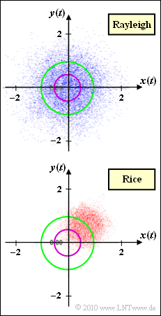
The graph shows the complex factor  $z(t) = x(t) + {\rm j} \cdot y(t)$  in the complex plane For the low-pass transmit signal  $s(t) = 1$ (which with respect to a bandpass–system corresponds to a cosine oscillation with amplitude  $1$ ), the low-pass receive signal  $r(t)$  is $z(t)$.

• The upper diagram describes  Rayleigh fading, where the component signals  $x(t)$  and  $y(t)$  are each Gaussian distributed with variance  $\sigma^2$. For  $a ≥ 0$, the probability density function of the magnitude  $a(t) = |z(t)|$  is:

$$f_a(a) = \frac{a}{\sigma^2} \cdot {\rm exp} [ -\frac{a^2 }{2\sigma^2}] \hspace{0.05cm}.$$

The noncentral second moment of  $z(t)$  is  $1$:

$${\rm E}\left [ |z(t)|^2 \right ] = 2 \sigma^2 = 1 \hspace{0.3cm} \Rightarrow \hspace{0.3cm} \sigma = {1}/{\sqrt{2}} \approx 0.707 \hspace{0.05cm}.$$

• The lower phase diagram is the result of  Rice fading. Here, too,   $x(t)$  and  $y(t)$  are Gaussian distributed with variance  $\sigma^2$, but now with mean value  $x_0$  and  $y_0$. The PDF for  $a ≥ 0$   is

$$f_a(a) = \frac{a}{\sigma^2} \cdot {\rm exp} \left[ -\frac{a^2 + |z_0|^2}{2\sigma^2}\right] \cdot {\rm I}_0 \left [ \frac{a \cdot |z_0|}{\sigma^2} \right ]\hspace{0.05cm}$$

where ${\rm I}_0$ is the modified Bessel function of the first kind.

The root mean square now includes the direct component  $z_0 = x_0 + {\rm j} \cdot y_0$

$${\rm E}\left [ |z(t)|^2 \right ] = 2 \cdot \sigma^2 + |z_0|^2 \hspace{0.05cm}.$$

For the system comparison

• the second moment is assumed to be constant: ${\rm E}\big[|z(t)|^2\big] = 1$,
• the Rice fading is based on the direction shown in the graph,
• let the power be split between the direct path  $(|z_0|^2)$  and the scattering paths  $(2\sigma^2)$  in the ratio  $4:1$ .

For the subtasks (1) to (4), let $s(t) = 1$. For the subtasks (5) or (6), a BPSK signal is assumed . The low-pass signal  $s(t)$  thus has a rectangular shape with the possible values  $±1$. The duration of each rectangular pulse is  $T = 10 \ \rm ms$.

Notes:

• This task belongs to chapter  Nichtfrequenzselektives Fading mit Direktkomponente.
• The circles drawn in the graph (violet and green) refer to the subtasks (3) and (4).

Questionnaire

1

How does the Rice–model result in an ideal channel   ⇒   $H(f) = 1$?

	With  $x_0 = y_0 = 0, \ \ \sigma^2 = 1$.
	With  $x_0 = 1, \ \ y_0 = 0, \ \ \ \sigma^2 = 0$.
	With  $x_0 = 0, \ \ \ y_0 = 1, \ \ \ \sigma^2 = 0$.

2

Determine the Rice–parameters used from the complex  $z(t)$–display on the details page.

$\sigma \ = \ $

$x_0 \ = \ $

$y_0 \ = \ $

3

What channel is  ${\rm Pr}(20 \cdot {\rm lg} \, |z(t)| ≤ -6 \ \ \rm dB)$  be bigger?

	On the present Rayleigh –channel
	In the case of this Rice–channel.
	The probabilities are approximately equal.

4

Which channel is used? Example: ${\rm Pr}(20 \cdot {\rm lg} \, |z(t)| ≤ 0 \ \ \rm dB)$  be bigger?

	On the present Rayleigh–channel
	In the case of this Rice–channel.
	The probabilities are approximately the same.

5

Which statements apply to a BPSK–transmit signal  $s(t)$  when considering the complex representation of the receive signal  $r(t)$ ?

	Rayleigh–Fading causes point clouds in quadrant  $1$  and  $3$.
	Rice–Fading will cause point clouds in quadrant  $1$  and  $3$.
	For Rayleigh, the WDF of  $|r(t)|$  is equal to the WDF of  $|z(t)|$.
	For Rice, the WDF of  $|r(t)|$  is equal to the WDF of  $|z(t)|$.

Sample solution

{ML Head (1)  Correct is the solution 2:

• The first suggestion returns a Rayleigh–fading–model. With the last setting the result would be

$$|z(t)| = {\rm j} \hspace{0.3cm}\Rightarrow \hspace{0.3cm} r(t) = s(t) \cdot z(t) = {\rm j} \cdot s(t) \hspace{0.05cm}.$$

• If we take into account that we are in the equivalent low-pass range, then a cosine input would produce a minus–sinusoidal output signal $r_{\rm BP}(t)$.
• On the other hand, solution 2 applies to all possible signals:

$$|z(t)| = x_0 = 1 \hspace{0.3cm}\Rightarrow \hspace{0.3cm} r(t) = s(t) \hspace{0.05cm}.$$

(2)  For the given Rayleigh–Fading the parameter $\sigma^2 = 0.5$. This results in $z(t)$ for the quadratic mean of the multiplicative factor: $${\rm E}\left [ |z(t)|^2 \right ] = 2 \sigma^2 = 1 \hspace{0.05cm}.$$

The Rice–Fading should have exactly the same performance. That is, it should apply: $$|z_0|^2 + 2 \sigma^2 = 1 \hspace{0.05cm}.$$

Furthermore, it was requested:

• The ratio of the power of the deterministic part ($|z_0|^2$) and the stochastic part ($2\sigma^2$) is $4$. It follows from this:

$$2 \sigma^2 \hspace{-0.1cm} \ = \ \hspace{-0.1cm} 0.2 \hspace{0.3cm}\Rightarrow \hspace{0.3cm} \sigma^2 = 0.1 \hspace{0.3cm}\Rightarrow \hspace{0.3cm} \sigma = \frac{1}{\sqrt{10}} \hspace{0.25cm} \underline{ \approx 0.316} \hspace{0.05cm},$$

$$|z_0|^2 \hspace{-0.1cm} \ = \ \hspace{-0.1cm} 0.8 \hspace{0.3cm}\Rightarrow \hspace{0.3cm} |z_0| = 0.894 \hspace{0.05cm}.$$

• The division of $z_0 = x_0 + {\rm j} \cdot y_0$ results from the graph. You can see that $y_0 = x_0$ (center of the cloud in the first quadrant below $45^\circ$):

$$x_0 = y_0 = \frac{|z_0|}{\sqrt{2}}} = \frac{0.894}{\sqrt{2}} \hspace{0.25cm} \underline{ \approx 0.632} \hspace{0.05cm}.$$

(3)  The range „$20 \cdot {\rm lg} \, |z(t)| ≤ \, –6 \ \ \rm dB$” is equal to „$|z(t)|≤0.5$”.

• This area is marked by the purple circle in the graph on the specifications page.
• You can see from this that the statement 1 is correct, because with Rayleigh there are more points within the violet circle.

Signal Section and WDF $f_a(a)$ for Rayleigh and Rice

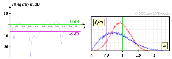
This graphic shows the result of a system simulation with the program „Mobile radio channel” from the (former) practical course „Simulation of digital transmission systems”.

• Both from the signal section as well as from the WDF one can see that the blue curve (Rayleigh) has more parts under the violet curve than the red curve (Rice).

(4)  Correct is solution 3:

• For the Rayleigh distribution the probability

$$${\rm Pr}(20 \cdot {\rm lg}\hspace{0.15cm} a(t) \le 0\,\,{\rm dB}) = {\rm Pr}(a(t) \le 1) = 1 - {\rm e}^{-1} \approx 63\,\,\ \hspace{0.05cm}.$$

• From the graph you can see that the probability for the riceversion (with the selected parameters) is about the same as the probability of falling below.
• This result can also be guessed from the complex representation of $z(t)$ on the data page (easier if you already know the result).
• Among other things, because the tip of the Gaussian cloud is still within the green circle.

Complex receive signal $r(t)$ for Rayleigh and Rice

(5)'  Correct are the solution proposals 2 and 3:

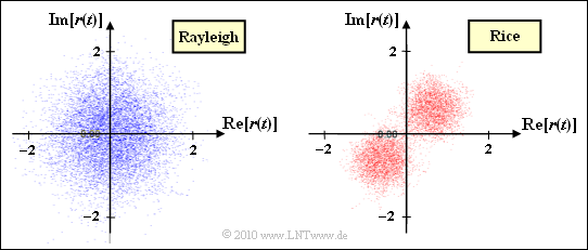
• At Rice–Fading the point cloud of $z(t)$ is in the first quadrant. If you multiply $z(t)$ by $s(t) = ±1$, you get two point clouds in the first and third quadrant. This does not change the WDF $f_a(a)$ of the amount.
• Even with Rayleigh–Fading the density functions $f_a(a)$ of the amount for $|z(t)|$ and $|r(t)|$ do not show any differences. Since the phase $\phi$ is equally distributed, the final result also has the same point clouds.
• However, if you look at the development of the complex representation of $z(t)$ and $r(t)$ dynamically, there are indeed differences.
• Larger jumps occur in the complex representation of $r(t)$, whenever there are phase jumps by $±180^\circ$ in the transmitted signal $s(t)$, i.e. when changing symbols.
• Thus, ${\it \Phi}_z(f_{\rm D})$ and ${\it \Phi}_r(f_{\rm D})$ &ndash are different for Rice–Fading; the latter is wider – and accordingly the corresponding autocorrelation function.

Translated with www.DeepL.com/Translator (free version)