Aufgaben:Exercise 2.5Z: Compression Factor vs. Residual Redundancy

• Return to book

Data length $L(N)$ after LZW coding for $\rm BQ1$ and $\rm BQ2$

As in  Exercise 2.5  we consider data compression using the  Lempel–Ziv–Welch algorithm. Here holds:

• Let the input sequence have the length  $N$.
• The length of the LZW coder output is  $L$.

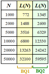
The graph shows for two different binary sources  $\rm BQ1$  and  $\rm BQ2$  the relationship between the sequence lengths  $N$  and  $L$,  represented by the function  $L(N)$. 

The two sources have the same statistical properties as in  Exercise 2.5:

• $\rm BQ1$  is redundant due to unequal symbol probabilities  $(p_{\rm A} = 0.89$  and  $p_{\rm B} = 0.11)$ .  There are no dependencies between the individual symbols.  The entropy is  $H = 0.5$ bit/source symbol.
• $\rm BQ2$  is redundancy-free and thus has the entropy  $H = 1$ bit/source symbol.

Furthermore, you need two definitions for the solution of this task:

• Let the  "compression factor"  be by definition

$$K(N) = \frac{L(N)}{N}\hspace{0.05cm}.$$

• The relative redundancy of the LZW code sequence  (called  "residual redundancy"  in the following)  is

$$r(N) = \frac{L(N) - N \cdot H}{L(N)}= 1 - \frac{ N \cdot H}{L(N)}\hspace{0.05cm}.$$

Hints:

• The exercise belongs to the chapter  Compression according to Lempel, Ziv and Welch.
• In particular, reference is made to the pages

Remainding redundancy as a measure of the efficiency of coding methods,

Efficiency of Lempel-Ziv coding and

Quantitative statements on asymptotic optimality.

Questions

1

Which compression factors  $K(N)$  result with  $N = 10000$?

$\rm BQ1$:     $K(N = 10000) \ = \ $

$\rm BQ2$:     $K(N = 10000) \ = \ $

2

What is the residual redundancy  $r(N)$  (in percent)?  Let  $N = 10000$ apply again.

$\rm BQ1$:     $r(N = 10000) \ = \ $ $\ \%$

$\rm BQ2$:     $r(N = 10000) \ = \ $ $\ \%$

3

What conclusions can be drawn from the comparison of  $N = 10000$  And  $N = 50000$?

	For both sources  $K(N = 50000)$  is smaller than  $K(N = 10000)$.
	For both sources  $r(N = 50000)$  is smaller than  $r(N = 10000)$.
	Only  $\rm BQ1$  has more favourable values with  $N = 50000$ .

Solution

Solution

(1)  The compression factor is defined as the quotient of the lengths of the LZW output sequence  $(L)$  and input sequence  $(N = 10000)$:

$${\rm BQ1:}\hspace{0.3cm} K \hspace{0.2cm} = \hspace{0.2cm} \frac{6800}{10000}\hspace{0.15cm}\underline{= 0.680}\hspace{0.05cm},$$

$$ {\rm BQ2:}\hspace{0.3cm} K \hspace{0.2cm} = \hspace{0.2cm} \frac{12330}{10000}\hspace{0.15cm}\underline{= 1.233}\hspace{0.05cm}. $$

• Of course, the LZW coding only makes sense with the redundant binary source  $\rm BQ1$ .  Here the amount of data can be reduced by  $32\%$ .
• With the redundancy-free binary source  $\rm BQ2$ , on the other hand, the LZW coding leads to a  $23.3\%$  larger data quantity.

(2)  From the given equation we obtain with  $N = 10000$:

$${\rm BQ1:}\hspace{0.3cm} H = 0.5\hspace{0.05cm},\hspace{0.2cm} r(N=10000) \hspace{0.2cm} = \hspace{0.2cm}1 - \frac{0.5 \cdot N}{L } = 1 - \frac{5000}{6800 } \hspace{0.15cm}\underline{\approx 26.5\,\%}\hspace{0.05cm},$$

$$ {\rm BQ2:}\hspace{0.3cm} H = 1.0\hspace{0.05cm},\hspace{0.2cm} r(N=10000) \hspace{0.2cm} = \hspace{0.2cm}1 - \frac{N}{L } = 1 - \frac{10000}{12330 } \hspace{0.15cm}\underline{\approx 19\,\%}\hspace{0.05cm}.$$

• The residual redundancy indicates the (relative) redundancy of the LZW output sequence.
• Although the source  $\rm BQ1$  is more suitable for LZW coding than the redundancy-free source  $\rm BQ2$,   $\rm BQ1$  results in a larger residual redundancy because of the redundancy in the input sequence.
• A smaller residual redundancy  $r(N)$  for a given  $N$  therefore says nothing about whether LZW coding is useful for the source at hand.
• For this, the compression factor  $K(N)$  must be considered.   In general, the following relationship between  $r(N)$  and  $K(N)$ applies:

$$r(N) = 1 - \frac{H}{K(N)}\hspace{0.05cm},\hspace{0.5cm} K(N) = H \cdot (1- r(N)) \hspace{0.05cm}.$$

(3)  From the table on the information page one can read  (or deduce)

• for the redundant binary source  $\rm BQ1$:

$$L(N = 50000) = 32100\hspace{0.05cm},\hspace{0.5cm} K(N = 50000) = 0.642\hspace{0.05cm},\hspace{0.5cm}r(N = 50000) \hspace{0.15cm}\underline {= 22.2\,\% \hspace{0.05cm}},$$

• for the redundancy-free binary source  $\rm BQ2$:

$$L(N = 50000) = 59595\hspace{0.05cm},\hspace{0.5cm} K(N = 50000) = 1.192\hspace{0.05cm},\hspace{0.5cm}r(N = 50000) \hspace{0.15cm}\underline {= 16.1\,\% \hspace{0.05cm}}.$$

Statements 1 and 2 are therefore correct:

• For both sources the compression factor  $K(N)$  is smaller for  $N = 50000$  than for  $N = 10000$.
• The same applies to the residual redundancy:   $r(N = 50000) < r(N = 10000)$.
• Both with regard to  $K(N)$  and  $r(N)$  "more favourable" values result with larger  $N$ , even if, as with the redundancy-free binary source  $\rm BQ2$ , the application of Lempel–Ziv actually leads to a deterioration.