Theory of Stochastic Signals/Further Distributions

1. Theory of Stochastic Signals
2. Continuous Random Variables
3. Further Distributions

• Previous page
• Next page

• Previous page
• Next page

Rayleigh PDF

$\text{Definition:}$  A continuous random variable  $x$  is called  Rayleigh distributed if it cannot take negative values and the probability density function (PDF) for  $x \ge 0$  with the distribution parameter  $λ$  has the following shape:

$$f_{x}(x)=\frac{x}{\lambda^2}\cdot {\rm e}^{-x^2 / ( 2 \hspace{0.05cm}\cdot \hspace{0.05cm}\lambda^2) } .$$

The name goes back to the English physicist  John William Strutt  the "third Baron Rayleigh".  In 1904 he received the physics–Nobel Prize.

• The Rayleigh distribution plays a central role in the description of time-varying channels.  Such channels are described in the book  Mobile Communications  .
• For example, non-frequency selective fading exhibits such a distribution when there is no line-of-sight between the base station and the mobile user.

Characteristic properties of Rayleigh distribution:

• A Rayleigh distributed random variable  $x$  cannot take negative values.
• The theoretically possible value  $x = 0$  also occurs only with probability "zero".
• The  $k$-th moment of a Rayleigh distributed random variable  $x$  results in general to

$$m_k=(2\cdot \lambda^{\rm 2})^{\it k/\rm 2}\cdot {\rm \Gamma}( 1+ {\it k}/{\rm 2}) \hspace{0.3cm}{\rm with }\hspace{0.3cm}{\rm \Gamma}(x)= \int_{0}^{\infty} t^{x-1} \cdot {\rm e}^{-t} \hspace{0.1cm}{\rm d}t.$$

• From this, the mean  $m_1$  and the rms  $\sigma_1$  can be calculated as follows:

$$m_1=\sqrt{2}\cdot \lambda\cdot {\rm \Gamma}(1.5) = \sqrt{2}\cdot \lambda\cdot {\sqrt{\pi}}/{2} =\lambda\cdot\sqrt{{\pi}/{2}},$$

$$m_2=2 \lambda^2 \cdot {\rm \Gamma}(2) = 2 \lambda^2 \hspace{0.3cm}\Rightarrow \hspace{0.3cm}\sigma = \sqrt{m_2 - m_1^2} =\lambda\cdot\sqrt{2-{\pi}/{2}}.$$

• To model a Rayleigh distributed random variable  $x$  one uses, for example, two Gaussian distributed, zero mean, and statistically independent random variables  $u$  and  $v$, both of which have rms  $σ = λ$  The variables  $u$  and  $v$  are then linked as follows:

$$x=\sqrt{u^2+v^2}.$$

Sample signal and PDF of a Rayleigh distributed random variable

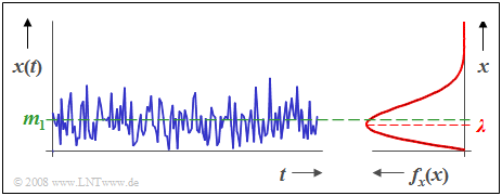
$\text{Example 1:}$  The graph shows:

• the time course  $x(t)$  of a Rayleigh distributed random variable as well as.
• the associated density function  $f_{x}(x)$.

One can see from this representation:

• The Rayleigh–PDF is always asymmetric.
• The mean  $m_1$  lies about  $25\%$  above the PDF maximum.
• The PDF maximum occurs at  $x = λ$ .

Rice PDF

Rice distribution also plays an important role in the description of time-varying channels, in part because,

• because  non-frequency selective fading  is Rice distributed if,
• if there is  line-of-sight'  between the base station and the mobile subscriber.

$\text{Definition:}$  A continuous random variable  $x$  is called  Rice distributed if it cannot take negative values and the probability density function (WDF) for  $x > 0$  has the following shape:

$$f_{\rm x}(x)=\frac{x}{\lambda^2}\cdot{\rm e}^{-({C^2+\it x^{\rm 2} })/ ({\rm 2 \it \lambda^{\rm 2} })}\cdot {\rm I_0}(\frac{\it x\cdot C}{\lambda^{\rm 2} }) \hspace{0.4cm}{\rm with} \hspace{0.4cm} {\rm I_0}(x) = \sum_{k=0}^{\infty}\frac{(x/2)^{2k} }{k! \cdot {\rm \gamma ({\it k}+1)} }.$$

${\rm I_0}( ... )$ denotes the  modified zero-order Bessel function.

The name is due to the mathematician and logician  Henry Gordon Rice . He taught as a mathematics professor at the University of New Hampshire.

Characteristic properties of the Rice distribution:

• The additional parameter  $C$  compared to the Rayleigh distribution is a measure of the "strength" of the direct component.  The larger the quotient  $C/λ$  is, the more the  Rice–channel approximates the Gaussian–channel.   For  $C = 0$  the Rice distribution transitions to the  Rayleigh distribution.
• In the Rice distribution, the expression for the moment  $m_k$  is much more complicated and can only be specified using hypergeometric functions.  However, if  $λ$  is much smaller than  $C$, then  $m_1 ≈ C$  and  $σ ≈ λ$ holds.
• Under these conditions, the Rice distribution can be approximated by a  Gaussian distribution  with mean  $C$  and rms  $λ$  .
• To model a Rice distributed random variable  $x$  we use a similar model as for the Rayleigh distribution, except that now at least one of the two Gaussian-distributed and statistically independent random variables  $(u$  and/or  $v$ )  must have a non-zero mean.

$$x=\sqrt{u^2+v^2}\hspace{0.5cm}{\rm with}\hspace{0.5cm}|m_u| + |m_v| > 0 .$$

Sample signal and PDF of a Rice distributed random variable

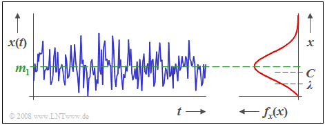
$\text{Example 2:}$  The graph shows the time course of a Rice distributed random variable  $x$  and its density function  $f_{\rm x}(x)$, where  $C/λ = 2$  holds.

• Somewhat casually put,   The Rice distribution is a compromise between the Rayleigh– and the Gaussian distributions.
• The mean  $m_1$  here is slightly larger than  $C$.

With the interactive applet  PDF, CDF and Moments of Special Distributions  you can display the characteristics  $($PDF, CDF, Moments$)$  of the Rayleigh– as well as the Rice distribution, among others.

Cauchy PDF

$\text{Definition:}$  A continuous random variable  $x$  is called  Cauchy distributed if the probability density function (PDF) and the distribution function (CDF) with distribution parameter  $λ$  have the following form:

$$f_{x}(x)=\frac{1}{\pi}\cdot\frac{\lambda}{\lambda^2+x^2},$$

$$F_{x}(r)={\rm 1}/{2}+{\rm arctan}({r}/{\lambda}).$$

Sometimes in the literature a mean  $m_1$  is also considered.

The name derives from the French mathematician  Augustin-Louis Cauchy , a pioneer of calculus who further developed the foundations established by  Gottfried Wilhelm Leibniz  and  Sir Isaac Newton  and formally proved fundamental propositions.  In particular, many central theorems of function theory derive from Cauchy.

The Cauchy distribution has less practical significance for communications engineering, but is mathematically very interesting.

It has the following properties in the symmetric form  $($with mean  $m_1 = 0)$  :

• For the Cauchy distribution, all moments  $m_k$  for even  $k$  have an infinitely large value, and this is independent of the parameter  $λ$.

• Thus, this distribution also has an infinitely large variance  $\sigma^2 = m_2$  ⇒  power.
• Thus, it is obvious that no physical variable can be Cauchy distributed.
• The quotient  $u/v$  of two independent Gaussian-distributed zero mean variable  $u$  and  $v$  is Cauchy distributed with the distribution parameter  $λ = σ_u/σ_v$  .
• A Cauchy distributed random variable  $x$  can be generated from a variable  $\pm1$  uniformly distributed between  $u$  by the following  nonlinear transformation :

$$x=\lambda \cdot {\tan}( {\pi}/{2}\cdot u).$$

• Because of symmetry, for odd  $k$  all moments  $m_k = 0$, assuming the "Cauchy Principal Value".
• So the mean value  $m_X = 0$  and the Charlier skewness  $S_X = 0$ also hold.

PDF of a Cauchy distributed random variable

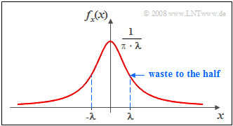
$\text{Example 3:}$  The graph shows the typical course of the Cauchy PDF.

• The slow decline of this function towards the edges can be seen.
• As this occurs asymptotically with  $1/x^2$  the variance and all higher order moments (with even index) are infinite.

Chebyshev's inequality

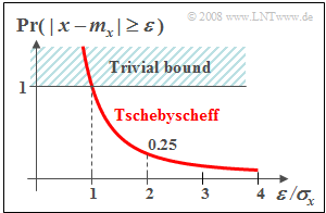
Given a random variable  $x$  with known probability density function  $f_{x}(x)$  the probability that the random variable  $x$  deviates in amount by more than one value  $ε$  from its mean  $m_{x}$  can be calculated exactly according to the way generally described in this chapter.

Chebyshev's inequality

• If besides the mean  $m_{x}$  the rms  $σ_{x}$  is known, but not the exact PDF course  $f_{x}(x)$, at least an upper bound can be given for this probability:

$${\rm Pr}(|x - m_{\rm x}|\ge\varepsilon)\le\frac{\sigma_{x}^{\rm 2}}{\varepsilon^{\rm 2}}. $$

• This bound given by  Pafnuti L. Chebyshev  - known as "Chebyshev's inequality" - is in general, however, only a very rough approximation for the actual exceeding probability.  It should therefore be applied only in the case of an unknown course of the PDF  $f_{x}(x)$  .

$\text{Example 4:}$  We assume a Gaussian distributed and zero mean random variable  $x$  .

• Thus, the probability that its absolute value  $\vert x \vert $  is greater than three times the rms  $(3 - σ_{x})$  is easily computable.  Result:  ${\rm 2 - Q(3) ≈ 2.7 - 10^{-3} }.$
• Tschebyshev's inequality yields here as an upper bound the clearly too large value  $1/9 ≈ 0.111$.
• This Chebyshev bound would also hold for any PDF form.

Exercises for the chapter

Exercise 3.10: Rayleigh Fading

Exercise 3.10Z: Rayleigh? Or Rice?

Exercise 3.11: Chebyshev's Inequality

Exercise 3.12: Cauchy Distribution