Aufgaben:Exercise 3.5: Triangular and Trapezoidal Signal

• Return to book

rectangle signal,  triangle signal
and trapezoid signal

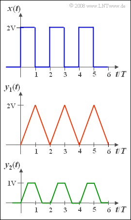
We start from the rectangular signal  $x(t)$  according to the upper graph.

• The amplitude values are  $0\hspace{0.05cm} \rm V$  and  $2\hspace{0.05cm} \rm V$.
• Let the duration of a rectangle and the distance between two successive rectangular pulses be equal to each  $T$.
• The random variable  $x$  – the instantaneous value of the rectangular signal  $x(t)$  – thus has the characteristic values  (mean,  rms value):

$$m_x = \sigma_x = 1\hspace{0.05cm} \rm V.$$

If we now apply this signal to a linear filter with the impulse response

$$h_{\rm 1}(t)=\left \{ \begin{array}{*{4}{c}} 1/T & {\; \rm for}\hspace{0.2cm}{ 0\le t \le T} \\\ 0 & {\rm else} \end{array} \right. , $$

then the triangular signal  $y_1(t) = x(t) \star h_1(t)$  is obtained at its output according to the convolution with

• the minimum values  $0\hspace{0.05cm} \rm V$  $($at  $t = 0,  2T,  4T, $ ...$)$,
• the maximum values  $2\hspace{0.05cm} \rm V$  $($at  $t = T,  3T,  5T, $ ...$)$.

Thus, this low-pass filter is an integrator over the time duration  $T$.

If,  on the other hand,  we apply the signal   $x(t)$  to the input of a filter with the impulse response

$$h_{\rm 2}(t)=\left \{ \begin{array}{*{4}{c}} 1/T & {\; \rm for}\hspace{0.2cm}{ 0\le t \le T/2} \\\ 0 & {\rm else} \end{array} \right. , $$

so the trapezoidal signal  $y_2(t) = x(t) \star h_2(t)$.  This second filter thus acts as an integrator over the time duration  $T/2$.

Hints:

• This exercise belongs to the chapter  Uniformly distributed random variables.

• For the corresponding frequency responses  $H_1(f=0)= 1$  or  $H_2(f=0)= 0.5$.

Questions

1

Which of the following statements are true?

	$y_1(t)$  is a continuous valued random variable.
	$y_1(t)$  has a triangular PDF.
	$y_1(t)$  is uniformly distributed.
	$y_2(t)$  has continuous and discrete valued components.

2

How large is the uniform part of the signal  $y_1(t)$?  Check this value  $m_{y1}$  also by using the variables  $m_x$  and  $H_1(f=0)$.

$m_{y1} \ = \ $ $\ \rm V$

3

Determine the power of the signal  $y_1(t)$  by both time averaging and coulter averaging.

$P_{y1} \ = \ $ $\ \rm V^2$

4

What is the rms value of the signal  $y_1(t)$?

$\sigma_{y1} \ = \ $ $\ \rm V$

5

What is the probability that  $y_1(t)$  is larger than  $0.75\hspace{0.05cm} \rm V$?

${\rm Pr}(y_1 > 0.75\hspace{0.05cm} \rm V) \ = \ $ $ \ \%$

6

Determine the PDF of the signal  $y_2(t)$  and sketch it.  As a check, enter the PDF value at the point  $y_2 = 0.5\hspace{0.05cm} \rm V$.

$f_{y2}(y_2= 0.5\hspace{0.05cm} \rm V) \ = \ $ $\ \rm 1/V$

7

What is the DC component of the signal  $y_2(t)$?  Check this value  $m_{y2}$  also using the quantities  $m_x$  and  $H_2(f=0)$.

$m_{y2} \ = \ $ $\ \rm V$

8

What is the rms value of the signal  $y_2(t)$?

$\sigma_{y2} \ = \ $ $\ \rm V$

9

What is the probability that  $y_2(t)$  is larger than  $0.75\hspace{0.05cm} \rm V$?

${\rm Pr}(y_2 > 0.75\hspace{0.05cm} \rm V) \ = \ $ $ \ \%$

Solution

Solution

Amplitude limit, 
readable in the PDF

(1)  Correct are  the proposed solutions 1, 3 and 4:

• The random variable  $y_1$  is uniformly distributed and thus just like  $x$  also a continuous valued random variable.
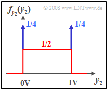
• The PDF of  $y_2$  exhibits discrete proportions at  $0\hspace{0.05cm} \rm V$  and  $2\hspace{0.05cm} \rm V$  on.
• There are,  of course,  continuous valued components between these two boundaries. 
• In this domain holds  $f_{y2}(y_2) = 1/2$.

(2)  The linear mean  $m_x = 1\hspace{0.05cm} \rm V$  can be read directly from the data sketch,  but could also be formally calculated using the equation for the uniform distribution $($between  $0\hspace{0.05cm} \rm V$  and  $2\hspace{0.05cm} \rm V)$.  Another solution is provided by the relation:

$$m_{y_{\rm 1}}=m_x\cdot H_{\rm 1}( f= 0) = 1\hspace{0.05cm} \rm V \cdot 1 \hspace{0.15cm}\underline{ =\rm 1\hspace{0.05cm} \rm V}.$$

(3)  Actually,  the averaging should be done over the whole time domain (both sides to infinity).

• However,  for reasons of symmetry,  the averaging over the time interval  $0 \le t \le T$  is sufficient:

$$P_{y_{\rm 1}}=\rm\frac{1}{\it T}\cdot \int_{\rm 0}^{\it T} \hspace{-0.15cm}\it y_{\rm 1}{\rm (}\it t{\rm {\rm )}}^{\rm 2}\it \hspace{0.05cm}\hspace{0.1cm}{\rm d}t=\rm\frac{1}{\it T}\cdot \int_{\rm 0}^{\it T} \hspace{-0.15cm}(\rm 2V \cdot \it\frac{t}{T}{\rm )}^{\rm 2} \hspace{0.1cm}{\rm d} t = \rm {4}/{3}\, V^2 \hspace{0.15cm}\underline{= \rm 1.333\, V^2}.$$

• Sharp averaging gives the same result.  Using the PDF  $f_{y1}(y_1) = 1/(2\hspace{0.05cm} \rm V)$  namely:

$$P_{y_{\rm 1}}= \int_0^{2V} \hspace{-0.3cm}\it y_{\rm 1}^{\rm 2}\cdot f_{\it y_{\rm 1}}{\rm (}\it y_{\rm 1}{\rm )}\it \hspace{0.1cm}{\rm d}y_{\rm 1} =\rm\frac{1}{2V}\cdot \int_0^{2V} \hspace{-0.3cm}\it y_{\rm 1}^{\rm 2}\hspace{0.1cm}{\rm d}y_{\rm 1} =\rm \frac{8\,{\rm V^3}}{3 \cdot 2\,{\rm V}} \hspace{0.15cm}\underline{= \rm 1.333\, V^2}.$$

(4)  The variance can be determined using Steiner's theorem:

$$4/3\hspace{0.05cm} \rm V^2 - 1\hspace{0.05cm} \rm V^2 = 1/3\hspace{0.05cm} \rm V^2.$$

• The root of this is the standard deviation  (rms value)  we are looking for:    

$$\sigma_{y_{\rm 1}}\hspace{0.15cm}\underline{=0.577 \, \rm V}.$$

(5)  The probability we are looking for is the integral over the PDF of  $0.75\hspace{0.05cm} \rm V$  to $2\hspace{0.05cm} \rm V$, i.e.

$${\rm Pr}(y_1 > 0.75\hspace{0.05cm} \rm V) \hspace{0.15cm}\underline{ = 62.5\%}.$$

(6)  The PDF consists of two Dirac delta functions at  $0\hspace{0.05cm} \rm V$  and  $1\hspace{0.05cm} \rm V$  $($each with weight  $1/4)$  and a constant continuous component of

$$f_{y2}(y_2= 0.5\hspace{0.05cm} \rm V) \hspace{0.15cm}\underline{=0.5 \cdot\rm 1/V}.$$

• At  $y_2 = 0.5 \hspace{0.05cm} \rm V$  there is therefore only the continuous part.

(7)  The mean value  $m_{y_{\rm 2}}\hspace{0.15cm}\underline{ =\rm 0.5\hspace{0.05cm} \rm V}$  can be read directly from the above PDF sketch or calculated as in subtask  (2)  as follows:

$$m_{y_{\rm 2}} = m_x\cdot H_{\rm 2}( f = 0) = 1\hspace{0.05cm} \rm V \cdot 0.5 {\hspace{0.1cm} = \rm 0.5\hspace{0.05cm} \rm V}.$$

(8)  With the above PDF,  for given power:

$$P_{y_{\rm 2}}=\int_{-\infty}^{+\infty}\hspace{-0.3cm}y_{\rm 2}^{\rm 2}\cdot f_{\it y_{\rm 2}}{\rm (}\it y_{\rm 2})\hspace{0.1cm}{\rm d}y_{\rm 2}=\rm \frac{1}{2}\cdot\frac{1}{3}\cdot 1\,V^2+\rm \frac{1}{4}\cdot 1\,V^2 = 5/12 \,V^2 \hspace{0.15cm}{ =\rm 0.417\,V^2}.$$

• The first part goes back to the continuous PDF,  the second part to the PDF Dirac function at  $1\hspace{0.05cm} \rm V$.
• The Dirac function at  $0\hspace{0.05cm} \rm V$  does not contribute to the power.  It follows for the rms value:

$$\sigma_{y_{\rm 2}} = \sqrt{{\rm 5}/{\rm 12}\rm V^2 -{1}/{4}\rm V^2}= \sqrt{{\rm 1}/{\rm 6}\rm V^2} \hspace{0.15cm}\underline{=0.409\, \rm V}.$$

(9)  This probability is also composed of two parts:

$${\rm Pr}(y_2 > 0.75 {\rm V} ) = {\rm Pr}(0.75 {\rm V} \le y_2 < 1 {\rm V} ) + {\rm Pr}(y_2 = 1 {\rm V} ) = \frac{1}{2} \cdot \frac{1}{4}+ \frac{1}{4} = \frac{3}{8}\hspace{0.15cm}\underline{ = 37.5\%}. $$