Aufgaben:Exercise 3.3Z: Moments for Triangular PDF

• Return to book

Two triangular PDFs

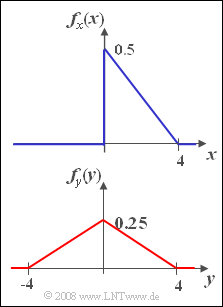
We consider in this exercise two random signals  $x(t)$  and  $y(t)$  each with triangular PDF,  namely

• the one-sided triangular PDF according to the upper graph:

$$f_x(x)=\left\{ \begin{array}{*{4}{c}} 0.5 \cdot (1-{ x}/{\rm 4}) & \rm for\hspace{0.2cm}{\rm 0 \le {\it x} \le 4},\\\rm 0 & \rm else. \end{array} \right.$$

• the two-sided triangular PDF according to the graph below:

$$ f_y(y)=\left\{ \begin{array}{*{4}{c}} 0.25 \cdot (1-{ |y|}/{\rm 4}) & \rm for\hspace{0.2cm}{ -4 \le {\it y} \le \rm 4},\\\rm 0 & \rm else. \end{array} \right.$$

To solve this problem,  consider the equation for the central moments:

$$\mu_k=\sum\limits_{\kappa = \rm 0}^{\it k}\left({k} \atop {\kappa}\right)\cdot m_k\cdot(-m_{\rm 1})^{k - \kappa}.$$

Specifically,  this equation yields the following results:

$$\mu_{\rm 1}=0,\hspace{0.5cm}\mu_{\rm 2}=\it m_{\rm 2}-\it m_{\rm 1}^{\rm 2},\hspace{0.5cm}\mu_{\rm 3}=\it m_{\rm 3}-\rm 3\cdot\it m_{\rm 2}\cdot \it m_{\rm 1} {\rm +}\rm 2\cdot\it m_{\rm 1}^{\rm 3},$$

$$\mu_{\rm 4}=\it m_{\rm 4}-\rm 4\cdot\it m_{\rm 3}\cdot \it m_{\rm 1}\rm +6\cdot\it m_{\rm 2}\cdot\it m_{\rm 1}^{\rm 2}-\rm 3\cdot\it m_{\rm 1}^{\rm 4}.$$

From the central moments of higher order one can derive among others:

• the  "Charlier's skewness"  $S = {\mu_3}/{\sigma^3}\hspace{0.05cm},$

• the  "kurtosis"  $K = {\mu_4}/{\sigma^4}\hspace{0.05cm}.$

Hints:

• This exercise belongs to the chapter  Expected Values and Moments.
• Reference is made to the section  Some common central moments.

Questions

1

Calculate from the present PDF  $f_x(x)$  the  $k$-th order moment.  What value results for the linear mean  $m_x = m_1$?

$m_x \ = \ $

2

What is the quadratic mean and the rms  $\sigma_x$  of the random variable  $x$?

$\sigma_x\ = \ $

3

For random variable  $x$:  What is the Charlier's skewness  $S_x = \mu_3/\sigma_x^3$?  Why is  $S_x \ne 0$?

$S_x \ = \ $

4

Which statements are true for the symmetrically distributed random variable  $y$?

	All moments with odd  $k$  are  $m_k =0$.
	All moments with even  $k$  are  $m_k =0$.
	All moments  $m_k$  with even  $k$  are calculated as in subtask  (1).
	The central moments   $\mu_k$  are equal to the non-centered moments  $m_k$.

5

Calculate the standard deviation of the random variable  $y$.

$\sigma_y \ = \ $

6

What is the kurtosis  $K_y$  of the random variable  $y$?  Interpret the result.

$K_y \ = \ $

Solution

Solution

(1)  For the  $k$–th order moment of the random variable  $x$  holds:

$$m_k=1/2\cdot \int_{\rm 0}^{\rm 4} x^k\cdot ( 1-\frac{\it x}{\rm 4}) \hspace{0.1cm}{\rm d}x.$$

• This leads to the result:

$$m_k=\frac{x^{ k+ 1}}{ 2\cdot ( k+ 1)}\Bigg|_{\rm 0}^{\rm 4}-\frac{x^{ k+2}}{8\cdot ( k+2)}\Bigg|_{\rm 0}^{\rm 4}=\frac{\rm 2\cdot \rm 4^{\it k}}{(\it k\rm +1)\cdot (\it k\rm + 2)}.$$

• From this we obtain for the linear mean  $(k= 1)$:

$$m_x=\rm {4}/{3}\hspace{0.15cm}\underline{=1.333}.$$

(2)  The  $(k= 2)$  is  $m_2 = 8/3$.

• From this follows with  "Steiner's theorem":

$$\sigma_x^{\rm 2}={8}/{3}-({4}/{3})^2=\rm {8}/{9}\hspace{0.5cm}\Rightarrow\hspace{0.5cm} \sigma_x\hspace{0.15cm}\underline{\approx \rm 0.943}.$$

(3)  With  $m_1 = 4/3$,  $m_2 = 8/3$  and  $m_3 = 32/5$,  the given equation for the third order central moment gives:   $\mu_3 = 64/135 \approx 0.474$.

• From this follows for the  "Charlier's skewness":

$$S_x=\rm \frac{64/135}{\Big(\sqrt {8/9}\Big)^3}=\frac{\sqrt{8}}{5}\hspace{0.15cm}\underline{\approx 0.566}.$$

• Due to the asymmetric PDF:  $S_x \ne 0$.

(4)  Correct are  the proposed solutions 1, 3 and 4:

• For symmetric PDF,  all odd moments are zero,  including the mean  $m_y$.
• Therefore,  according  $y$:  There is no difference between the moments  $m_k$  and the central moments  $\mu_k$.
• The moments  $m_k$  with even  $k$  are the same for the random variables  $x$  and  $y$.  This is evident from the time averages:
• Since  $x^2(t) = y^2(t)$,  for  $k = 2n$  the moments are equal too:

$$m_k=m_{2 n}=\ \text{...}\int [x^2(t)]^n \hspace{0.1cm}{\rm d} x=\ \text{...}\int [y^2(t)]^n \hspace{0.1cm}{\rm d} y.$$

(5)  With the result of the subtask  (2)  holds:

$$m_2=\mu_{\rm 2}=\sigma_y^2=\rm {8}/{3} = 2.667\hspace{0.3cm}\Rightarrow\hspace{0.3cm} \sigma_y\hspace{0.15cm}\underline{=1.633}.$$

(6)  For symmetrical PDF,  the fourth-order central moment is equal to the moment  $m_4$.

• From the general equation calculated in subtask  (1)  one obtains  $\mu_4 = 256/15.$
• From this follows for the kurtosis:

$$K_y=\frac{\mu_{\rm 4}}{\sigma_y^{\rm 4}}=\rm \frac{256/15}{(8/3)^2}\hspace{0.15cm}\underline{=2.4}.$$

Note:   This numerical value is valid for the triangle PDF in general and lies between the kurtosis values of the uniform distribution  $(K = 1.8)$  and the Gaussian distribution  $(K = 3)$. This is a quantitative evaluation of the fact that here

• the outliers are more pronounced than in the case of a uniformly distributed random size,
• but due to the limitation less pronounced than with Gaussian sizes.

• Then we will prove that the asymmetric triangular PDF  $f_x(x)$  has the same kurtosis as shown in the upper sketch on the data sheet:

$$\mu_{ 4} = m_{\rm 4}- 4\cdot m_{\rm 3}\cdot m_{\rm 1}+ 6\cdot m_{\rm 2}\cdot m_{\rm 1}^{\rm 2}- 3\cdot m_{\rm 1}^{\rm 4}= \frac{256}{15} - 4 \cdot \frac{32}{5}\cdot \frac{4}{3} + 6 \cdot \frac{8}{3}\cdot \left(\frac{4}{3}\right)^2 -3 \cdot \left(\frac{4}{3}\right)^4 =\frac{256}{15 \cdot 9}$$

• With the result of the subtask  (3)    ⇒   $\sigma_x^2 = 8/9$  it follows:

$$ K_x = \frac{{256}/(15 \cdot 9)}{8/9 \cdot 8/9} = 2.4.$$