Difference between revisions of "Aufgaben:Exercise 4.11: C Program "acf1""
From LNTwww
| Line 4: | Line 4: | ||
[[File:P_ID391__Sto_A_4_11.png|right|frame|C program $1$ for ACF–calculation '''correction''']] | [[File:P_ID391__Sto_A_4_11.png|right|frame|C program $1$ for ACF–calculation '''correction''']] | ||
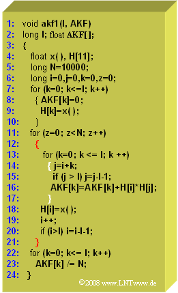
| − | See the C–program " | + | See the C–program "acf1" for calculating the discrete ACF values $\varphi_x(k)$ with index $k = 0$, ... , $l$. The following should be noted about this: |
* Let the long–value passed to the program $l = 10$. The ACF values $\varphi_x(0)$, ... , $\varphi_x(10)$ are returned to the calling program with the float field $\rm ACF\big[ \ \big]$ . In lines 7 and 8 of the program given on the right, this field is pre-populated with zeros. | * Let the long–value passed to the program $l = 10$. The ACF values $\varphi_x(0)$, ... , $\varphi_x(10)$ are returned to the calling program with the float field $\rm ACF\big[ \ \big]$ . In lines 7 and 8 of the program given on the right, this field is pre-populated with zeros. | ||
| Line 10: | Line 10: | ||
* The random variables to be analyzed $x_\nu$ are generated with the float function $x( \ )$ (see line 4). This function is called a total of $N + l + 1 = 10011$ times (lines 9 and 18). | * The random variables to be analyzed $x_\nu$ are generated with the float function $x( \ )$ (see line 4). This function is called a total of $N + l + 1 = 10011$ times (lines 9 and 18). | ||
| − | * In contrast to the algorithm given in the [[Theory_of_Stochastic_Signals/Auto-Correlation_Function#Numerical_ACF_determination|Theory section]] program " | + | * In contrast to the algorithm given in the [[Theory_of_Stochastic_Signals/Auto-Correlation_Function#Numerical_ACF_determination|Theory section]] program "acf2" of [[Aufgaben:Exercise_4.11Z:_C_Program_"acf2"|Task 4.11Z]] directly implemented, one needs here an auxiliary field ${\rm H}\big[ \ \big]$ with only $l + 1 = 11$ memory elements. |
Revision as of 14:43, 6 March 2022
See the C–program "acf1" for calculating the discrete ACF values $\varphi_x(k)$ with index $k = 0$, ... , $l$. The following should be noted about this:
- Let the long–value passed to the program $l = 10$. The ACF values $\varphi_x(0)$, ... , $\varphi_x(10)$ are returned to the calling program with the float field $\rm ACF\big[ \ \big]$ . In lines 7 and 8 of the program given on the right, this field is pre-populated with zeros.
- The random variables to be analyzed $x_\nu$ are generated with the float function $x( \ )$ (see line 4). This function is called a total of $N + l + 1 = 10011$ times (lines 9 and 18).
- In contrast to the algorithm given in the Theory section program "acf2" of Task 4.11Z directly implemented, one needs here an auxiliary field ${\rm H}\big[ \ \big]$ with only $l + 1 = 11$ memory elements.
- Before starting the actual calculation algorithm (lines 11 to 21), the eleven memory cells of ${\rm H}\big[ \ \big]$ contain the random values $x_1$, ... , $x_{11}$.
- The outer loop with the index $z$ (marked in red) is run $N$ times.
- In the inner loop (marked white) with the index $k = 0$, ... , $l$ all memory cells of the field ${\rm ACF}\big[\hspace{0.03cm} k \hspace{0.03cm} \big]$ are increased by the contribution $x_\nu \cdot x_{\nu+k}$ .
- Finally, in lines 22 and 23, all ACF–values are divided by the number $N$ of data analyzed.
Hint:
- This exercise belongs to the chapter Auto-Correlation Function.
- Reference is made in particular to the page Numerical ACF determination.
Questions
Solution
(1) With $z= 0$ and $k=6$ results according to the program: $\underline{i= 0}$ and $\underline{j= 6}$.
- The corresponding memory contents are ${\rm H}\big[\hspace{0.03cm} 0 \hspace{0.03cm}\big] = x_1$ and ${\rm H}\big[\hspace{0.03cm} 6 \hspace{0.03cm}\big] = x_7$.
(2) In the field ${\rm H}\big[\hspace{0.03cm} 0 \hspace{0.03cm}\big]$ the random variable $x_{12}$ is now entered:
- $$\text{memory cell }\underline{i= 0},\hspace{1cm}\text{sequence index }\underline{\nu= 12}.$$
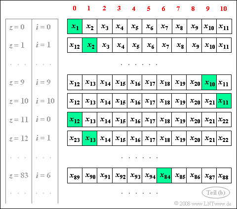
(3) The graph shows the allocation of the auxiliary field with the random values $x_\nu$.
- In each case, the memory cell is highlighted in green ${\rm H}\big[\hspace{0.03cm} i \hspace{0.03cm}\big]$. The new random variable is entered into this memory location at the end of each loop (line 18).
- For $z= 83$ and $K=6$ this results in.
- $$\underline{i= 83 \hspace{-0.2cm}\mod \hspace{-0.15cm} \ 11 = 6},\hspace{1cm} \underline{j= (i+k)\hspace{-0.2cm}\mod \hspace{-0.15cm} \ 11 = 1}.$$
- Loop pass $z= 83$: In memory cell ${\rm H}\big[\hspace{0.03cm} 6 \hspace{0.03cm}\big]$ is the random variable $x_{84}$ and in the memory cell ${\rm H}\big[\hspace{0.03cm} 1 \hspace{0.03cm}\big]$ is the random variable $x_{90}$.
- At the end of the loop pass $z= 83$ in ${\rm H}\big[\hspace{0.03cm} 6 \hspace{0.03cm}\big]$ the content $x_{84}$ is replaced by $x_{95}$ .

