Difference between revisions of "Aufgaben:Exercise 4.6: Quantization Characteristics"
From LNTwww
| Line 3: | Line 3: | ||
}} | }} | ||
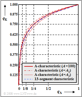
| − | [[File: | + | [[File:EN_Mod_A_4_6_neu.png|right|frame|Non-linear quantization characteristics]] |
Non-linear quantization is considered. The system model according to [[Aufgaben:Exercise_4.5:_Non-Linear_Quantization| Exercise 4.5]] still applies. | Non-linear quantization is considered. The system model according to [[Aufgaben:Exercise_4.5:_Non-Linear_Quantization| Exercise 4.5]] still applies. | ||
Latest revision as of 15:01, 11 April 2022
Non-linear quantization is considered. The system model according to Exercise 4.5 still applies.
The graph shows two compressor characteristics $q_{\rm K}(q_{\rm A})$:
- Drawn in red is the so-called "A-characteristic" recommended by the CCITT ("Comité Consultatif International Téléphonique et Télégraphique") for the standard system PCM 30/32. For $0 ≤ q_{\rm A} ≤ 1$ applies here:
- $$q_{\rm K}(q_{\rm A}) = \left\{ \begin{array}{l} \frac{1 \hspace{0.05cm}+\hspace{0.05cm} {\rm ln}(A \hspace{0.05cm}\cdot \hspace{0.05cm}q_{\rm A})} {1 \hspace{0.05cm}+ \hspace{0.05cm}{\rm ln}(A )} \\ \\ \frac{A \hspace{0.05cm}\cdot \hspace{0.05cm}q_{\rm A}} {1 \hspace{0.05cm}+ \hspace{0.05cm}{\rm ln}(A )} \\ \end{array} \right.\quad \begin{array}{*{10}c} {{1}/{A} \le q_{\rm A} \le 1} \hspace{0.05cm}, \\ \\ {q_{\rm A} < {1}/{A}} \hspace{0.05cm}. \\ \end{array}$$
- The blue-dashed curve applies to the so-called "13-segment characteristic". This is obtained from the A-characteristic by piecewise linearization; it is treated in detail in the Exercise 4.5 .
Hints:
- The Exercise belongs to the chapter "Pulse Code Modulation".
- Reference is made in particular to the page "Compression and Expansion".
- For the A-characteristic drawn in solid red, the quantization parameter $A = 100$ is chosen. With the value $A = 87.56$ suggested by CCITT, a similar curve is obtained.
- For the other two curves,
- $A = A_1$ (dash–dotted curve) and
- $A = A_2$ (dotted curve),
where for $A_1$ and $A_2$ the two possible numerical values $50$ and $200$ are given. In the subtask (3) you are to decide which curve belongs to which numerical value.
Questions
Solution
(1) Correct are the statements 2 and 3:
- Signal distortion of soft sounds or in speech pauses is subjectively perceived as more disturbing than e.g. additional noise in heavy metal.
- In terms of quantization noise or SNR, however, there is no improvement due to non-linear quantization if an uniformly distribution of the amplitude values is assumed.
- However, if one considers that in speech and music signals smaller amplitudes occur much more frequently than large ⇒ "Laplace distribution", non-linear quantization also results in a better SNR.
(2) Correct are the statements 1 and 2:
- Due to the linearization in the individual segments, the interval width of the various quantization levels is constant in these for the "13-segment characteristic", which has a favorable effect in realization.
- In contrast, with the non-linear quantization according to the "A-characteristic", there are no quantization intervals of equal width.
This means: The statement 3 is false.
(3) Correct is "NO":
- For $q_{\rm A} = 1$ one obtains independently of $A$ the value $q_{\rm K} = 1$.
- So with this specification alone $A$ cannot be determined.
(4) Correct is again "NO":
- For $q_{\rm A} = 1/A$ both range equations yield the same value $q_{\rm K}= 1/[1 + \ln(A)]$.
- Also with this $A$ cannot be determined.
(5) With this requirement $A$ is now computable:
- $$0.875 = \frac{1 \hspace{0.05cm}+\hspace{0.05cm} {\rm ln}(A/2)} {1 \hspace{0.05cm}+ \hspace{0.05cm}{\rm ln}(A )} = \frac{1\hspace{0.05cm}-\hspace{0.05cm} {\rm ln}(2) \hspace{0.05cm}+\hspace{0.05cm} {\rm ln}(A)} {1 \hspace{0.05cm}+ \hspace{0.05cm}{\rm ln}(A )}\approx \frac{1-0.693 \hspace{0.05cm}+\hspace{0.05cm} {\rm ln}(A)} {1 \hspace{0.05cm}+ \hspace{0.05cm}{\rm ln}(A )}\hspace{0.3cm} \Rightarrow \hspace{0.3cm}{\rm ln}(A) = \frac{0.875 - 0.307 } {1 -0.875 }= 4.544 \hspace{0.3cm}\Rightarrow \hspace{0.3cm} A \hspace{0.15cm}\underline {\approx 94} \hspace{0.05cm}.$$
(6) Correct is statement 2:
- The curve for $A_1 = 200$ lies above the curve with $A = 100$, the curve with $A_2 = 50$ below.
- This is shown by the following calculation for $q_{\rm A} = 0.5$:
- $$A= 100\text{:}\hspace{0.2cm} q_{\rm K}= \frac{1 + \ln(100) - \ln(2)}{1 + \ln(100)}= \frac{1+4.605- 0.693} {1 +4.605}\approx 0.876 \hspace{0.05cm},$$
- $$A= 200\text{:}\hspace{0.2cm} q_{\rm K}= \frac{1+5.298- 0.693} {1 +5.298}\approx 0.890 \hspace{0.05cm},$$
- $$A= 50\text{:}\hspace{0.4cm} q_{\rm K}= \frac{1+3.912- 0.693} {1 +3.912}\approx 0.859 \hspace{0.05cm}.$$
