Aufgaben:Exercise 4.4Z: Supplement to Exercise 4.4

• Return to book

Hamming weights and sequence probabilities

The information theorist  "Robert G. Gallager"  already in 1963 dealt with the following problem:

• Given a random vector  $\underline{x} = (x_1, \, x_2, \hspace{-0.04cm} \text{ ...} \hspace{0.08cm} , x_n)$  with  $n$  binary elements  $x_i ∈ \{0, \, 1\}$.
• Known are all probabilities  $p_i = {\rm Pr}(x_i = 1)$  and  $q_i = {\rm Pr}(x_i = 0) = 1 - p_i$  with index  $i = 1, \hspace{-0.04cm}\text{ ...} \hspace{0.08cm} ,\ n$.
• What we are looking for is the probability that the number of ones in this vector is even.
• Or expressed using the  "Hamming weight":   What is the probability  ${\rm Pr}[w_{\rm H}(\underline{x}) {\rm \ is \ even}]$?

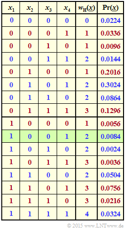
The graph illustrates the task for the example  $n = 4$  and  $p_1 = 0.2$,  $p_2 = 0.9$,  $p_3 = 0.3$  and  $p_4 = 0.6$.

• For the row highlighted in green   ⇒   $\underline{x} = (1, \, 0, \, 0, \, 1)$  holds  $w_{\rm H}(\underline{x}) = 2$  and

$${\rm Pr}(\underline{x}) = p_1 \cdot q_2 \cdot q_3 \cdot p_4 = 0.0084.$$

• Blue font means "$w_{\rm H}(\underline{x})$ is even". Red font stands for "$w_{\rm H}(\underline{x})$ is odd."
• The probability  ${\rm Pr}[w_{\rm H}(\underline{x}) {\rm \ is \ even}]$  is the sum of the blue numbers in the last column.
• The sum of the red numbers gives  ${\rm Pr}[w_{\rm H}(\underline{x}) {\rm \ is \ odd}] = 1 - {\rm Pr}[w_{\rm H}(\underline{x}) {\rm \ is \ even}]$.

Gallager solved the problem in an analytical way:

$${\rm Pr} \left [w_{\rm H}(\underline{x})\hspace{0.15cm}{\rm is \hspace{0.15cm} even} \right ] \hspace{-0.15cm} \ = \ \hspace{-0.15cm} 1/2 \cdot [1 + \pi]\hspace{0.05cm},$$

$${\rm Pr} \left [w_{\rm H}(\underline{x})\hspace{0.15cm}{\rm is \hspace{0.15cm} odd} \right ] \hspace{-0.15cm} \ = \ \hspace{-0.15cm} 1/2 \cdot [1 - \pi]\hspace{0.05cm}.$$

Here the following auxiliary variable is used:

$$\pi = \prod\limits_{i =1}^{n} \hspace{0.25cm}(1-2p_i) \hspace{0.05cm}.$$

One applies the equation, for example, to calculate the extrinsic  $L$–values of a  single parity–check code .

Indeed, as already pointed out in  "Exercise A4.4"  the extrinsic $L$–value with Hamming–weight  $w_{\rm H}$  is the truncated sequence  $\underline{x}^{(-i)}$:

$$L_{\rm E}(i) = {\rm ln} \hspace{0.15cm}\frac{{\rm Pr} \left [w_{\rm H}(\underline{x}^{(-i)})\hspace{0.15cm}{\rm ist \hspace{0.15cm} gerade} \hspace{0.05cm} | \hspace{0.05cm}\underline{y} \hspace{0.05cm}\right ]}{{\rm Pr} \left [w_{\rm H}(\underline{x}^{(-i)})\hspace{0.15cm}{\rm ist \hspace{0.15cm} ungerade} \hspace{0.05cm} | \hspace{0.05cm}\underline{y} \hspace{0.05cm}\right ]} \hspace{0.05cm}.$$

Here it is taken into account that for  $L_{\rm E}(i)$  one may refer only to the other symbols  $(j ≠ i)$ :

$$\underline{x}^{(-i)} = \big ( \hspace{0.03cm}x_1, \hspace{-0.04cm} \text{ ...} \hspace{0.08cm} , \hspace{0.03cm} x_{i-1}, \hspace{0.43cm} x_{i+1}, \hspace{-0.04cm} \text{ ...} \hspace{0.08cm} , x_{n} \hspace{0.03cm} \big )\hspace{0.03cm}.$$

Hints:

• This exercise belongs to the chapter  "Soft–in Soft–out Decoder".
• Reference is made in particular to the page  "For calculating the extrinsic  $L$–values".
• The exercise is intended as a supplement to  "Exercise 4.4" .

Questions

1

We consider the vector  $\underline{x} = (x_1, \, x_2) \ \Rightarrow \ n = 2$  with  $x_i ∈ \{0, \, 1\}$  and  $p_1 = 0.2, \ p_2 = 0.9$.
What is the probability that  $\underline{x}$  contains an even number of ones?

${\rm Pr}\big [w_{\rm H}(\underline{x}) \ {\rm is \ even}\big ] \ = \ $

2

Berechnen Sie die gleiche Wahrscheinlichkeit für  $\underline{x} = (x_1, \, x_2, \, x_3) \ \Rightarrow \ n = 3$  und  $p_1 = 0.2, \ p_2 = 0.9, \ p_3 = 0.3$.

${\rm Pr}\big [w_{\rm H}(\underline{x}) \ {\rm is \ even}\big ] \ = \ $

3

Now let  $n = 4$  and  $p_1 = 0.2, \ p_2 = 0.9, \ p_3 = 0.3, \ p_4 = 0.6$. Calculate the following quantities according to Gallager's equation:

${\rm Pr(blue) = Pr}\big [w_{\rm H}(\underline{x}) \ {\rm is \ even}\big ] \hspace{0.33cm} = \ $

${\rm Pr(red) = Pr}\big [w_{\rm H}(\underline{x}) \ {\rm is \ odd}\big ] \hspace{0.1cm} = \ $

$\text{Quotient }Q = {\rm Pr(blau)/Pr(rot)} \hspace{0.4cm} = \ $

4

What is the extrinsic  $L$ value for the symbol  $i = 5$  at  $\text{SPC (5, 4, 2)}$  with  $p_1 = 0.2, \ p_2 = 0.9, \ p_3 = 0.3, \ p_4 = 0.6, \ p_5 = 0.9$?

$L_{\rm E}(i = 5) \ = \ $

5

How does  $L_{\rm E}(i = 5)$ change if we assume  $p_5 = 0.1$  instead?

	$L_{\rm E}(i = 5)$  becomes larger.
	$L_{\rm E}(i = 5)$  becomes smaller.
	$L_{\rm E}(i = 5)$  is not changed compared to subtask (4).

Solution

Solution

Derivation "$w_{\rm H}$ is even" for code length $n = 2$.

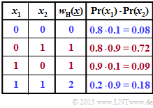
(1)  According to the adjacent table applies:

$${\rm Pr} \left [w_{\rm H}(\underline{x})\hspace{0.10cm}{\rm is \hspace{0.10cm} even}\right ] = {\rm Pr} \left [w_{\rm H} = 0 \right] + {\rm Pr} \left [w_{\rm H} = 2 \right] \hspace{0.05cm}.$$

With the probabilities

$$p_1 = {\rm Pr} (x_1 = 1) \hspace{-0.15cm} \ = \ \hspace{-0.15cm} 0.2\hspace{0.05cm},\hspace{0.3cm}q_1 = {\rm Pr} (x_1 = 0) = 0.8\hspace{0.05cm},$$

$$p_2 = {\rm Pr} (x_2 = 1) \hspace{-0.15cm} \ = \ \hspace{-0.15cm} 0.9\hspace{0.05cm},\hspace{0.3cm}q_2 = {\rm Pr} (x_2 = 0) = 0.1$$

one obtains:

$${\rm Pr} \left [w_{\rm H}(\underline{x}) = 0\right] \hspace{-0.15cm} \ = \ \hspace{-0.15cm} {\rm Pr} \left [(x_1 = 0)\cap (x_2 = 0) \right] = q_1 \cdot q_2 = 0.8 \cdot 0.1 = 0.08 \hspace{0.05cm},$$

$${\rm Pr} \left [w_{\rm H}(\underline{x}) = 2\right] \hspace{-0.15cm} \ = \ \hspace{-0.15cm} {\rm Pr} \left [(x_1 = 1)\cap (x_2 = 1) \right] = p_1 \cdot p_2 = 0.2 \cdot 0.9 = 0.18$$

$$\Rightarrow \hspace{0.3cm} {\rm Pr} \left [w_{\rm H}(\underline{x})\hspace{0.15cm}{\rm is \hspace{0.15cm} even}\right] = 0.8 + 0.18 \hspace{0.15cm} \underline{= 0.26} \hspace{0.05cm}.$$

The Gallager's equation provides for the same set of parameters:

$${\rm Pr} \left [w_{\rm H}(\underline{x})\hspace{0.15cm}{\rm is \hspace{0.15cm} even}\right] \hspace{-0.15cm} \ = \ \hspace{-0.15cm} 0.5 + 0.5 \cdot \prod\limits_{i =1}^{2} \hspace{0.25cm}(1-2\cdot p_i) = 0.5 + 0.5 \cdot (1 - 2 \cdot 0.2)\cdot (1 - 2 \cdot 0.9) = 0.26 \hspace{0.05cm}.$$

The equation given by Gallager 1963 was hereby verified for $n = 2$.

Derivation "$w_{\rm H}$ is even" for code length $n = 3$.

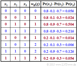
(2)  In the second table, the four combinations with an even number of ones are marked in blue. The probabilities of occurrence of each combination are given in the last column. Thus, the result is:

$${\rm Pr} \left [w_{\rm H}(\underline{x})\hspace{0.15cm}{\rm is \hspace{0.15cm} even}\right] = 0.056 + 0.216 + 0.006 + 0.126 \hspace{0.15cm} \underline{= 0.404} \hspace{0.05cm}.$$

The red rows provide the complementary event:

$${\rm Pr} \left [w_{\rm H}(\underline{x})\hspace{0.15cm}{\rm is \hspace{0.15cm} odd}\right] = 0.024 + 0.504 + 0.014 + 0.054= 0.596 \hspace{0.05cm}.$$

The Gallager's equation again gives the exact same result, although it should be noted that this equation is valid for all $n$ and all arbitrary probabilities:

$${\rm Pr} \left [w_{\rm H}(\underline{x})\hspace{0.15cm}{\rm is \hspace{0.15cm} even}\right] \hspace{-0.15cm} \ = \ \hspace{-0.15cm} 0.5 + 0.5 \cdot \prod\limits_{i =1}^{3} \hspace{0.25cm}(1-2\cdot p_i)$$

$$\Rightarrow\hspace{0.3cm}{\rm Pr} \left [w_{\rm H}(\underline{x})\hspace{0.15cm}{\rm is \hspace{0.15cm} even}\right] \hspace{-0.15cm} \ = \ \hspace{-0.15cm} 0.5 + 0.5 \cdot (+0.6) \cdot (-0.8) \cdot (+0.4) = 0.404 \hspace{0.05cm}.$$

(3)  According to the specification page applies:

$$\pi = \prod\limits_{i =1}^{4} \hspace{0.25cm}(1-2\cdot p_i) \hspace{-0.15cm} \ = \ \hspace{-0.15cm} (1 - 2 \cdot 0.2) \cdot (1 - 2 \cdot 0.9) \cdot (1 - 2 \cdot 0.3) \cdot (1 - 2 \cdot 0.6)$$

$$\Rightarrow\hspace{0.3cm}\pi = \prod\limits_{i =1}^{4} \hspace{0.25cm}(1-2\cdot p_i) \hspace{-0.15cm} \ = \ \hspace{-0.15cm}(+0.6) \cdot (-0.8) \cdot (+0.4) \cdot (-0.2) = 0.0384 \hspace{0.05cm}.$$

From this can be calculated:

$${\rm Pr}({\rm blue}) = {\rm Pr} \left [w_{\rm H}(\underline{x})\hspace{0.15cm}{\rm is \hspace{0.15cm} even}\right] \hspace{-0.15cm} \ = \ \hspace{-0.15cm} 0.5 + 0.5 \cdot \pi = 0.5 + 0.5 \cdot 0.0384\hspace{0.15cm} \underline{= 0.5192}\hspace{0.05cm},$$

$${\rm Pr}({\rm red}) = {\rm Pr} \left [w_{\rm H}(\underline{x})\hspace{0.15cm}{\rm is \hspace{0.15cm} odd}\right] \hspace{-0.15cm} \ = \ \hspace{-0.15cm} 0.5 - 0.5 \cdot \pi = 0.5 - 0.5 \cdot 0.0384\hspace{0.15cm} \underline{= 0.4808}\hspace{0.05cm}.$$

If you add up the blue and red probabilities on the information page, you get exactly the values calculated here.

For the quotient we get:

$$Q = \frac{{\rm Pr} \left [w_{\rm H}(\underline{x})\hspace{0.15cm}{\rm is \hspace{0.15cm} even}\right]} { {\rm Pr} \left [w_{\rm H}(\underline{x})\hspace{0.15cm}{\rm is \hspace{0.15cm} odd}\right]} = \frac{0.5192}{0.4808}\hspace{0.15cm} \underline{= 1.0799} \hspace{0.05cm}.$$

(4)  For the single parity–check code, the extrinsic $L$ value with respect to the $i$th bit was specified as follows:

$$L_{\rm E}(i) = {\rm ln} \hspace{0.15cm}\frac{{\rm Pr} \left [w_{\rm H}(\underline{x}^{(-i)})\hspace{0.15cm}{\rm is \hspace{0.15cm} even} \hspace{0.05cm} | \hspace{0.05cm}\underline{y} \hspace{0.05cm}\right ]}{{\rm Pr} \left [w_{\rm H}(\underline{x}^{(-i)})\hspace{0.15cm}{\rm is \hspace{0.15cm} odd} \hspace{0.05cm} | \hspace{0.05cm}\underline{y} \hspace{0.05cm}\right ]} \hspace{0.05cm},$$

or:

$$L_{\rm E}(i) = {\rm ln} \hspace{0.15cm}\frac{1+\prod_{j \ne i} \hspace{0.25cm}(1-2\cdot p_j)}{1-\prod_{j \ne i} \hspace{0.25cm}(1-2\cdot p_j)} \hspace{0.05cm}.$$

At  $\text{SPC (5, 4, 2}$)   ⇒   $n = 5$, this product for $i = 5$ results from the following four factors:

$$\pi = \prod\limits_{j = 1, \hspace{0.05cm}2, \hspace{0.05cm}3, \hspace{0.05cm}4} \hspace{0.05cm}(1-2\cdot p_j) = (1-2\cdot p_1) \cdot (1-2\cdot p_2) \cdot (1-2\cdot p_3) \cdot (1-2\cdot p_4) \hspace{0.05cm}.$$

The comparison with the subtask (3) shows that $L_{\rm E}(i = 5) = \ln {Q} = \ln {(1.0799)} \ \underline{\approx 0.077}$.

(5)  Correct is proposed solution 3 because the result for $L_{\rm E}(i = 5)$ is independent of $p_5$.