Aufgaben:Exercise 3.13: Path Weighting Function again

• Return to book

For the reduction of the state transition diagram

In the  "rules for manipulating the state transition diagram"  section, for the example of our rate 1/2 standard code with memory  $m = 2$  and the transfer function matrix

$${\boldsymbol{\rm G}}(D) = \big ( 1 + D + D^2\hspace{0.05cm},\hspace{0.1cm} 1 + D^2 \hspace{0.05cm}\big )$$

the calculation of path weighting enumerator functions was described in great detail. The results given were:

$$T_{\rm enh}(X, U) \hspace{-0.2cm} \ = \ \hspace{-0.2cm} \frac{U\hspace{-0.05cm} X^5}{1- 2U\hspace{-0.05cm}X} =U\hspace{-0.05cm}X^5 \cdot \big [ 1 + (2U\hspace{-0.08cm}X) + (2U\hspace{-0.08cm}X)^2 + \text{...} \hspace{0.05cm} \big ] \hspace{0.01cm},$$

$$T(X) \hspace{-0.2cm} \ = \ \hspace{-0.2cm} \frac{X^5}{1- 2X} = X^5 \cdot \big [ 1 + (2X) + (2X)^2 + \text{...} \hspace{0.05cm} \big ] \hspace{0.05cm}.$$

Now the same calculations shall be done for the  "equivalent systematic code"  with the transfer function matrix

$${\boldsymbol{\rm G}}(D) = \big ( 1 \hspace{0.05cm},\hspace{0.1cm} (1 + D^2)/(1 + D + D^2) \hspace{0.05cm}\big )$$

can be performed.

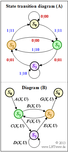
• The diagram shows the state transition diagram  $\rm (A)$  and the structure of the reduced diagram  $\rm (B)$, where the transitions are denoted by  $A(X, \, U), \ \text{...}\ , \ G(X, \, U)$  in general.
• In the subtask (1) these abbreviations are to be adapted to the state transition diagram  $\rm (A)$  .

Hints:

• This exercise belongs to the chapter  "Distance Characteristics and Error Probability Barriers".
• For the solution of the subtasks (2) and (3)' we refer here again to the section  "Rules for manipulating the state transition diagram" in the theory section.

Solution

1

What expressions do the following abbreviations stand for?

	$A(X, \, U) = UX^2$,
	$B(X, \, U) = UX$,
	$C(X, \, U) = X$,
	$D(X, \, U) = UX$,
	$E(X, \, U) = X$,
	$F(X, \, U) = 1$,
	$G(X, \, U) = UX^2$.

2

What expressions apply to the extended path weighting enumerator function?

	$T_{\rm enh}(X, \, U) = UX^5 \ / \ (1 \, –2UX)$.
	$T_{\rm enh}(X, \, U) = UX^5 + 2 U^2X^6 + 4U^3X^7 + 8U^4X^8 + \ \text{...}$,
	None of the proposals are correct.

3

What expressions apply to the "simple" path weighting enumerator function?

	$T(X) = X^5 \ / \ (1 \, –2X)$.
	$T(X) = X^5 + 2X^6 + 4X^7 + 8X^8 + \ \text{...}$
	None of the proposals are correct.

Solution

Solution

(1)  All proposed solutions are correct. In the adapted diagram  $\rm (B)$  all transitions are drawn:

Reduction of the state transition diagram

• The transition from $S_0$ to $S_1$ is denoted by "$1 \ | \ 11$".
• The output sequence $\underline{x}_i = (11)$ is expressed by $X^2$, the input bit $u_i = 1$ by $U$.
• The same result is obtained for $G(X, \, U)$:

$$A(X, U) = G(X, U)= UX^2 \hspace{0.05cm}.$$

• The output sequences $\underline{x}_i = (01)$ as well as $\underline{x}_i = (10)$ are both marked with $X$.
• Taking into account the input bits, we thus obtain:

$$u_i = 1\hspace{-0.1cm}:\hspace{0.15cm} B(X, U) = D(X, U)= UX\hspace{0.05cm},$$

$$u_i = 0\hspace{-0.1cm}:\hspace{0.15cm} C(X, U) = E(X, U)= X \hspace{0.05cm}.$$

• The transition "$0 \ | \ 00$" from $S_2$ to $S_1$ is expressed by $F(X, \, U) = 1$.

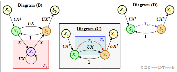
(2)  According to the procedure in section "Rules for manipulating the state transition diagram" in the theory section, first the transition from $S_1$ to $S_2$ via $S_3$ is summarized by an ring.

• One obtains for the red background in the diagram  $\rm (B)$:

$$T_1(X, U) = \frac{A(X, U) \cdot B(X, U)}{1- C(X, U)} = \frac{X \cdot X}{1- U \cdot X} \hspace{0.05cm}.$$

• The two parallel transitions corresponding to the blue background in the diagram  $\rm (C)$  can be combined as follows:

$$T_2(X, U) \hspace{-0.15cm} \ = \ \hspace{-0.15cm} T_1(X, U) + B(X, U) =\frac{X^2}{1- U X}+ U X = \frac{X^2 + U- U^2X^2}{1- U X} \hspace{0.05cm}.$$

• The extended path weighting enumerator function results according to diagram  $\rm (D)$  as feedback:

$$T_{\rm enh}(X, U) = \frac{A(X, U) \cdot G(X, U)\cdot T_2(X, U)}{1- F(X, U) \cdot T_2(X, U)} = \frac{UX^2 \cdot UX^2\cdot \frac{X^2 + UX- U^2X^2}{1- U X}}{1- 1 \cdot \frac{X^2 + UX- U^2X^2}{1- U X}}\hspace{0.05cm}.$$

Even after several attempts, the author has not succeeded in further simplifying this expression in a target-oriented way. He tends to the proposed solution 3 with the addition "without guarantee".

• However, this result would imply that the extended path weighting enumerator function of the equivalent systematic code is different from that of the nonsystematic code.
• We will still clarify this issue with an expert.

(3)  Correct are the proposed solutions 1 and 2:

• If one sets the formal parameter $U = 1$ in the extended function $T_{\rm enh}(X, \, U)$, one obtains the solution proposition 1:

$$T(X) = \frac{X^4 \cdot \frac{X^2 + X- X^2}{1- X}}{1- \frac{X^2 + X- X^2}{1- X}}= \frac{X^5 }{1- X - X} = \frac{X^5 }{1- 2X} \hspace{0.05cm}.$$

• Using the series expansion $1/(1 \, –x) = 1 + x + x^2 + \ \text{...}\ $, we arrive at the proposed solution 2.
• That is, the simple path weighting enumerator function $T(X)$ matches for both codes.