Channel Coding/The Basics of Product Codes

1. Channel Coding
2. Iterative Decoding Methods
3. The Basics of Product Codes

• Previous page
• Next page

• Previous page
• Next page

Basic structure of a product code

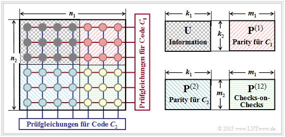
The graphic shows the principle structure of  »product codes«,  which were already introduced in 1954 by  $\text{Peter Elias}$. 

• The  two-dimensional product code  $\mathcal{C} = \mathcal{C}_1 × \mathcal{C}_2$  shown here is based on the two linear and binary block codes with parameters  $(n_1, \ k_1)$  and  $(n_2, \ k_2)$ respectively.

• The code word length is  $n = n_1 \cdot n_2$.

The  $n$  encoded bits can be grouped as follows:

Basic structure of a product code

• The  $k = k_1 \cdot k_2$  information bits are arranged in the  $k_2 × k_1$ matrix  $\mathbf{U}$.

• The code rate is equal to the product of the code rates of the base codes:

$$R = k/n = (k_1/n_1) \cdot (k_2/n_2) = R_1 \cdot R_2.$$

• The upper right matrix  $\mathbf{P}^{(1)}$  with dimension  $k_2 × m_1$  contains the parity bits with respect to the code  $\mathcal{C}_1$.

• In each of the  $k_2$  rows,  $m_1 = n_1 - k_1$  check bits are added to the  $k_1$  information bits as described in an earlier chapter using the example of  "Hamming codes" .
  

• The lower left matrix  $\mathbf{P}^{(2)}$  of dimension  $m_2 × k_1$  contains the check bits for the second component code  $\mathcal{C}_2$.  Here the encoding  $($and also the decoding$)$  is done line by line:   In each of the  $k_1$  columns,  the  $k_2$  information bits are still supplemented by  $m_2 = n_2 -k_2$  check bits.
  

• The  $m_2 × m_1$–matrix  $\mathbf{P}^{(12)}$  on the bottom right is called  "checks–on–checks".  Here the two previously generated parity matrices  $\mathbf{P}^{(1)}$  and  $\mathbf{P}^{(2)}$  are linked according to the parity-check equations.
  
  

$\text{Conclusions:}$  All product codes  according to the above graph have the following properties:

• For linear component codes  $\mathcal{C}_1$  and  $\mathcal{C}_2$  the product code  $\mathcal{C} = \mathcal{C}_1 × \mathcal{C}_2$  is also linear.
  

• Each row of  $\mathcal{C}$  returns a code word of  $\mathcal{C}_1$  and each column returns a code word of  $\mathcal{C}_2$.
  

• The sum of two rows again gives a code word of  $\mathcal{C}_1$ due to linearity.
  

• Also,  the sum of two columns gives a valid code word of  $\mathcal{C}_2$.
  

• Each product code also includes the  "zero word"  $\underline{0}$  $($a vector of  $n$  "zeros"$)$.
  

• The minimum distance of  $C$  is  $d_{\rm min} = d_1 \cdot d_2$,  where  $d_i$  indicates the minimum distance of  $\mathcal{C}_i$ 

Iterative syndrome decoding of product codes

We now consider the case where a product code with matrix  $\mathbf{X}$  is transmitted over a binary channel. 

• Let the received matrix  $\mathbf{Y} = \mathbf{X} + \mathbf{E}$, where  $\mathbf{E}$  denotes the  "error matrix".

• Let all elements of the matrices  $\mathbf{X}, \ \mathbf{E}$  and  $\mathbf{Y}$  be binary,  that is  $0$  or  $1$.
  

For the decoding of the two component codes the syndrome decoding according to the chapter  "Decoding linear block codes"  is suitable. 

In the two-dimensional case this means:

1. One first decodes the  $n_2$  rows of the received matrix  $\mathbf{Y}$,  based on the parity-check matrix  $\mathbf{H}_1$  of the component code  $\mathcal{C}_1$. 
   Syndrome decoding is one way to do this.
   
2. For this one forms in each case the so-called  "syndrome"   $\underline{s} = \underline{y} \cdot \mathbf{H}_1^{\rm T}$,  where the vector   $\underline{y}$   of length  $n_1$  indicates the current row of  $\mathbf{Y}$  and 
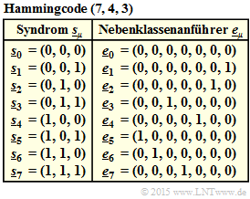
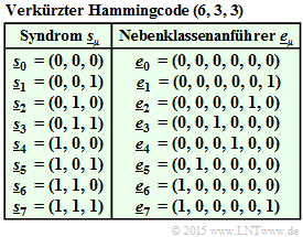
   "T"  stands for "transposed".
3. Correspondingly to the calculated  $\underline{s}_{\mu}$   $($with  $0 ≤ \mu < 2^{n_1 -k_1})$   one finds in a prepared syndrome table the corresponding probable error pattern  $\underline{e} = \underline{e}_{\mu}$.
   
4. If there are only a few errors within the row,  then   $\underline{y} + \underline{e}$   matches the sent row vector  $\underline{x}$. 
5. However,  if too many errors have occurred,  then incorrect corrections will occur.
   
6. Afterwards one decodes the  $n_1$  columns of the  $($corrected$)$  received matrix  $\mathbf{Y}\hspace{0.03cm}'$,  this time based on the  $($transposed$)$  parity-check matrix  $\mathbf{H}_2^{\rm T}$  of the component code  $\mathcal{C}_2$.
7. For this,  one forms the syndrome   $\underline{s} = \underline{y}\hspace{0.03cm}' \cdot \mathbf{H}_2^{\rm T}$,  where the vector  $\underline{y}\hspace{0.03cm}'$  of length  $n_2$  denotes the considered column of  $\mathbf{Y}\hspace{0.03cm}'$  .
   
8. From a second syndrome table  $($valid for code  $\mathcal{C}_2)$  we find for the computed  $\underline{s}_{\mu}$  $($with  $0 ≤ \mu < 2^{n_2 -k_2})$  the probable error pattern $\underline{e} = \underline{e}_{\mu}$ of the edited column.
9. After correcting all columns,  the matrix  $\mathbf{Y}$  is present.  Now one can do another row and then a column decoding   ⇒   second iteration,  and so on,  and so forth.
   
   

$\text{Example 1:}$  To illustrate the decoding algorithm,  we again consider the  $(42, 12)$  product code,  based on

• the Hamming code  $\text{HC (7, 4, 3)}$   ⇒   code  $\mathcal{C}_1$,
  

• the truncated Hamming code  $\text{HC (6, 3, 3)}$   ⇒   code  $\mathcal{C}_2$.
  

Syndrome decoding of the  $(42, 12)$  product code

Syndrome table for code $\mathcal{C}_1$

Syndrome table for the code $\mathcal{C}_2$

The left graph shows the received matrix  $\mathbf{Y}$. 

Note:   For display reasons, 

• the code matrix  $\mathbf{X}$  was chosen to be a  $6 × 7$ zero matrix, 

• so that the nine  "ones"  in  $\mathbf{Y}$  represent transmission errors
  

⇒   The  row-by-row syndrome decoding  is done via the syndrome  $\underline{s} = \underline{y} \cdot \mathbf{H}_1^{\rm T}$  with

$$\boldsymbol{\rm H}_1^{\rm T} = \begin{pmatrix} 1 &0 &1 \\ 1 &1 &0 \\ 0 &1 &1 \\ 1 &1 &1 \\ 1 &0 &0 \\ 0 &1 &0 \\ 0 &0 &1 \end{pmatrix} \hspace{0.05cm}.$$

In particular:

• Row 1  ⇒  Single error correction is successful  $($also in rows 3,  4 and 6$)$:

$$\underline{s} = \left ( 0, \hspace{0.02cm} 0, \hspace{0.02cm}1, \hspace{0.02cm}0, \hspace{0.02cm}0, \hspace{0.02cm}0, \hspace{0.02cm}0 \right ) \hspace{-0.03cm}\cdot \hspace{-0.03cm}{ \boldsymbol{\rm H} }_1^{\rm T} \hspace{-0.05cm}= \left ( 0, \hspace{0.03cm} 1, \hspace{0.03cm}1 \right ) = \underline{s}_3$$

$$\Rightarrow \hspace{0.3cm} \underline{y} + \underline{e}_3 = \left ( 0, \hspace{0.02cm} 0, \hspace{0.02cm}0, \hspace{0.02cm}0, \hspace{0.02cm}0, \hspace{0.02cm}0, \hspace{0.02cm}0 \right ) \hspace{0.05cm}.$$

• Row 2   $($contains two errors$)$   ⇒   Error correction concerning bit  5:

$$\underline{s} = \left ( 1, \hspace{0.02cm} 0, \hspace{0.02cm}0, \hspace{0.02cm}0, \hspace{0.02cm}0, \hspace{0.02cm}0, \hspace{0.02cm}1 \right ) \hspace{-0.03cm}\cdot \hspace{-0.03cm}{ \boldsymbol{\rm H} }_1^{\rm T} \hspace{-0.05cm}= \left ( 1, \hspace{0.03cm} 0, \hspace{0.03cm}0 \right ) = \underline{s}_4$$

$$\Rightarrow \hspace{0.3cm} \underline{y} + \underline{e}_4 = \left ( 1, \hspace{0.02cm} 0, \hspace{0.02cm}0, \hspace{0.02cm}0, \hspace{0.02cm}1, \hspace{0.02cm}0, \hspace{0.02cm}1 \right ) \hspace{0.05cm}.$$

• Row 5  $($also contains two errors$)$  ⇒  Error correction concerning bit  3:

$$\underline{s} = \left ( 0, \hspace{0.02cm} 0, \hspace{0.02cm}0, \hspace{0.02cm}1, \hspace{0.02cm}1, \hspace{0.02cm}0, \hspace{0.02cm}0 \right ) \hspace{-0.03cm}\cdot \hspace{-0.03cm}{ \boldsymbol{\rm H} }_1^{\rm T} \hspace{-0.05cm}= \left ( 0, \hspace{0.03cm} 1, \hspace{0.03cm}1 \right ) = \underline{s}_3$$

$$\Rightarrow \hspace{0.3cm} \underline{y} + \underline{e}_3 = \left ( 0, \hspace{0.02cm} 0, \hspace{0.02cm}1, \hspace{0.02cm}1, \hspace{0.02cm}1, \hspace{0.02cm}0, \hspace{0.02cm}0 \right ) \hspace{0.05cm}.$$

⇒   The  column-by-column syndrome decoding  removes all single errors in columns  1,  2,  3,  4  and  7.

• Column 5  $($contains two errors$)$   ⇒   Error correction concerning bit  4:

$$\underline{s} = \left ( 0, \hspace{0.02cm} 1, \hspace{0.02cm}0, \hspace{0.02cm}0, \hspace{0.02cm}1, \hspace{0.02cm}0 \right ) \hspace{-0.03cm}\cdot \hspace{-0.03cm}{ \boldsymbol{\rm H} }_2^{\rm T} \hspace{-0.05cm}= \left ( 0, \hspace{0.02cm} 1, \hspace{0.02cm}0, \hspace{0.02cm}0, \hspace{0.02cm}1, \hspace{0.02cm}0 \right ) \hspace{-0.03cm}\cdot \hspace{-0.03cm} \begin{pmatrix} 1 &1 &0 \\ 1 &0 &1 \\ 0 &1 &1 \\ 1 &0 &0 \\ 0 &1 &0 \\ 0 &0 &1 \end{pmatrix} = \left ( 1, \hspace{0.03cm} 0, \hspace{0.03cm}0 \right ) = \underline{s}_4$$

$$\Rightarrow \hspace{0.3cm} \underline{y} + \underline{e}_4 = \left ( 0, \hspace{0.02cm} 1, \hspace{0.02cm}0, \hspace{0.02cm}1, \hspace{0.02cm}1, \hspace{0.02cm}0 \right ) \hspace{0.05cm}.$$

⇒   The remaining three errors are corrected by decoding the  second row iteration loop  $($line-by-line$)$.

Whether all errors of a block are correctable depends on the error pattern.  Here we refer to  $\text{Exercise 4.7}$

Performance of product codes

The 1954 introduced  product codes  were the first codes,  which were based on recursive construction rules and thus in principle suitable for iterative decoding.  The inventor Peter Elias did not comment on this,  but in the last twenty years this aspect and the simultaneous availability of fast processors have contributed to the fact that in the meantime product codes are also used in real communication systems, e.g.

• in error protection of storage media,  and

• in very high data rate fiber optic systems.
  

Usually one uses very long product codes   $($large  $n = n_1 \cdot n_2)$   with the following consequence:

• For effort reasons,  the  "maximum likelihood decoding at block level"  is not applicable for the component codes  $\mathcal{C}_1$  and  $\mathcal{C}_2$  nor the  "syndrome decoding",  which is after all a realization form of maximum likelihood decoding.

• Applicable,  on the other hand,  even with large  $n$  is the  "iterative symbol-wise MAP decoding".  The exchange of extrinsic and a-priori–information happens here between the two component codes.  More details on this can be found in  [Liv15].
  

Bit and block error probability of a  $(1024, 676)$  product code at AWGN

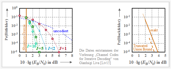
The graph shows for a  $(1024, 676)$  product code, based on the  extended Hamming code  ${\rm eHC} \ (32, 26)$  as component codes,

• on the left,  the bit error probability as function of the AWGN parameter  $10 \cdot {\rm lg} \, (E_{\rm B}/N_0)$  the number of iterations  $(I)$,

• on the right,  the error probability of the blocks,  $($or code words$)$.

Here are some additional remarks:

• The code rate is   $R = R_1 \cdot R_2 = 0.66$;  this results to the Shannon bound  $10 \cdot {\rm lg} \, (E_{\rm B}/N_0) \approx 1 \ \rm dB$.
  

• The left graph shows the influence of the iterations.  At the transition from  $I = 1$  to  $I=2$  one gains  $\approx 2 \ \rm dB$ $($at  $\rm BER =10^{-5})$  and with  $I = 10$  another  $\rm dB$.  Further iterations are not worthwhile.
  

• All bounds mentioned in the chapter  "Bounds for Block Error Probability"  can be applied here as well,  e.g. the   "truncated union bound"  $($dashed curve in the right graph$)$:

$${\rm Pr(Truncated\hspace{0.15cm}Union\hspace{0.15cm} Bound)}= W_{d_{\rm min}} \cdot {\rm Q} \left ( \sqrt{d_{\rm min} \cdot {2R \cdot E_{\rm B}}/{N_0}} \right ) \hspace{0.05cm}.$$

• The minimum distance is  $d_{\rm min} = d_1 \cdot d_2 = 4 \cdot 4 = 16$.  With the weight function of the  ${\rm eHC} \ (32, 26)$,

$$W_{\rm eHC(32,\hspace{0.08cm}26)}(X) = 1 + 1240 \cdot X^{4} + 27776 \cdot X^{6}+ 330460 \cdot X^{8} + ...\hspace{0.05cm} + X^{32},$$

we obtain for the product code:  $W_{d,\ min} = 1240^2 = 15\hspace{0.05cm}376\hspace{0.05cm}000$.

• This gives the block error probability bound shown in the graph on the right.
  

Exercises for the chapter

"Exercise 4.6: Product Code Generation"

"Exercise 4.6Z: Basics of Product Codes"

"Exercise 4.7: Product Code Decoding"

"Exercise 4.7Z: Principle of Syndrome Decoding"

References

- ↑ Liva, G.: Channels Codes for Iterative Decoding. Lecture manuscript, Department of Communications Engineering, TU Munich and DLR Oberpfaffenhofen, 2015.