Exercise 3.1Z: Triangular PDF
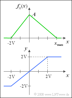
We consider a continuous random variable $x$ with the PDF outlined above.
- The minimum value of the signal is $x_{\rm min} = -2\hspace{0.05cm} {\rm V}$.
- On the other hand, the maximum value $x_{\rm max}$ is a free parameter, allowing values between $+2\hspace{0.05cm}\rm V$ and $+4\hspace{0.05cm} \rm V$ .
The random variable $x$ is to be understood here as the instantaneous value of a random signal. If this signal $x(t)$ is applied to an amplitude limiter with the characteristic curve (see sketch below)
$$y(t)=\left\{\begin{array}{*{4}{c}} -2\hspace{0.05cm} {\rm V} & {\rm if}\hspace{0.1cm} x(t)<-2\hspace{0.05cm} {\rm V} , \\ x(t) & {\rm if}\hspace{0.1cm}-2\hspace{0.05cm} {\rm V} \le x(t)\le +2\hspace{0.05cm} {\rm V}, \\ +2\hspace{0.05cm} {\rm V} & {\rm if}\hspace{0.1cm} {\it x}({\it t})>+2\hspace{0.05cm} {\rm V}, \\\end{array}\right.$$
so the signal $y(t)$ or the new random variable $y$, which is considered in the last two subquestions (5) and (6) is obtained.
- For the subtasks (1) and (2) apply $x_{\rm max} = 2\hspace{0.05cm} {\rm V} $.
- For all other subtasks, set $x_{\rm max} = 4\hspace{0.05cm} {\rm V} $ .
Hints:
- The task belongs to the chapter Probability Density Function.
- The topic of this chapter is illustrated with examples in the (German) learning video Wahrscheinlichkeit und WDF $\Rightarrow$ Probability and PDF.
Questions
Solution
(1) The area under the PDF must always yield the value $1$ . It follows that:
- $${A}/{ 2}\cdot {4\hspace{0.05cm}\rm V}=1\hspace{0.5cm}\Rightarrow\hspace{0.5cm} A \hspace{0.15cm}\underline{=\rm 0.5\;{1}/{V}}.$$
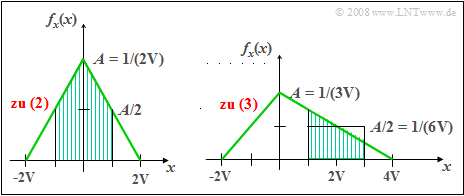
(2) With $x_{\rm max} = +2\hspace{0.05cm} {\rm V}$ the PDF is obtained according to the left graph.
- The shading marks the probability we are looking for.
- One obtains by simple geometric considerations:
- $${\rm Pr}(|x|<\rm 1\hspace{0.05cm} V)\hspace{0.15cm}\underline{=\rm 0.75}.$$
(3) With $x_{\rm max} = +4\hspace{0.05cm} {\rm V}$ one obtains the PDF shown on the right.
- The maximum value is now $A = 1/(3\hspace{0.05cm} {\rm V})$.
- The shaded area again indicates the probability we are looking for, which can be determined, for example, using the rectangle of equal area:
- $${\rm Pr}(1\hspace{0.05cm} {\rm V}< x<3\hspace{0.05cm} {\rm V})=\rm \frac{1}{6\hspace{0.05cm} {\rm V}}\cdot 2\hspace{0.05cm} {\rm V}=\hspace{0.15cm}\underline{0.333}.$$
(4) Since $x$ represents a continuous random variable, this probability is by definition zero ⇒ ${\rm Pr}(x =2\hspace{0.05cm} {\rm V}) \;\underline {= 0}$.
(5) Only the last statement of the given answers is true:
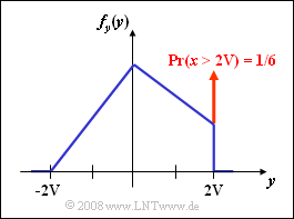
- The PDF $f_y(y)$ includes a continuous component (drawn in blue),
- but also the (red) Dirac function at $y = +2\hspace{0.05cm} {\rm V}$ with weight ${\rm Pr}(x >2\hspace{0.05cm} {\rm V})$.
(6) Opposite is the probability density of the random variable $y$ .
- From the right figure for the subtask (3) one can see the relation:
- $${\rm Pr}( y=2\hspace{0.05cm} {\rm V}) = {\rm Pr}( x> 2\hspace{0.05cm} {\rm V}) = \frac{1}{2}\cdot\frac{1}{6\hspace{0.05cm} {\rm V}}\cdot2{\hspace{0.05cm} {\rm V}} = {1}/{6}\hspace{0.15cm}\underline{=0.167}.$$


