Uniformly Distributed Random Variables

General description and definition

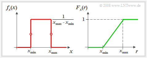
PDF and CDF of uniform distribution

$\text{Definition:}$ A random variable $x$ is said to be »uniformly distributed« if it can only take values in the range of $x_{\rm min}$ to $x_{\rm max}$ with equal probability.

The graph shows

on the left the probability density function $f_{x}(x)$,
right the cumulative distribution function $F_{x}(r)$

of such an equally distributed random variable $x$.

From the graph and this definition, the following properties can be derived:

The probability density function $\rm (PDF)$ has in the range from $x_{\rm min}$ to $x_{\rm max}$ the constant value $1/(x_{\rm max} - x_{\rm min})$.
On the range limits, only half the value - that is, the average value between the left–hand and right–hand limits - is to be set for $f_{x}(x)$ in each case.
The distribution function $\rm (CDF)$ increases linearly from $x_{\rm min}$ to $x_{\rm max}$ in the range from $0$ to $1$ .
Mean, variance and standard deviation (standard deviation) KORREKTUR: 2x standard deviation? of the uniform distribution have the following values:

$$m_{\rm 1} = \frac{\it x_ {\rm max} \rm + \it x_{\rm min}}{2},\hspace{0.5cm} \sigma^2 = \frac{[x_{\rm max} - x_{\rm min}]^2}{12},\hspace{0.5cm} \sigma = \frac{\it x_{\rm max} - \it x_{\rm min}}{2 \sqrt{3}}.$$

For symmetric PDF ⇒ $x_{\rm min} = -x_{\rm max}$ we obtain as a special case the mean $m_1 = 0$ and the variance $σ^2 = x_{\rm max}^2/3.$

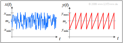
$\text{Example 1:}$ The graph shows two signal waveforms with uniform amplitude distribution.

Examples of uniformly distributed signals

On the left, statistical independence of the individual samples is assumed, that is, the random variable $x_ν$ can take all values between $x_{\rm min}$ and $x_{\rm max}$ with equal probability, and independently of the past $(x_{ν-1}, x_{ν-2}, \hspace{0.1cm}\text{...}).$

For the right signal $y(t)$ this independence of successive signal values is no longer given. Rather, this sawtooth signal represents a deterministic signal.

Importance of the uniform distribution for communications engineering

The importance of uniformly distributed random variables for information and communication technology is due to the fact that, from the point of view of information theory, this PDF form represents an optimum under the constraint $\text{peak limitation}$:

With no distribution other than the uniform distribution one achieves greater $\text{differential entropy}$ under this condition.
This topic is dealt with in the chapter "Differential Entropy" in the book "Information Theory".

$\text{In addition, the following points should be mentioned, among others:}$

(1) The importance of the uniform distribution for the simulation of communication systems is due to the fact that one can realize corresponding "pseudo-random generators" relatively easily, and that other distributions, such as the $\text{Gaussian distribution}$ and the $\text{exponential distribution}$ can be easily derived.

(2) In "Image Processing & Coding", simplifying calculations are often made using the uniform distribution instead of the actual distribution of the original image, which is usually much more complicated, since the difference in information content between a "natural image" and the model based on the uniform distribution is relatively small.

(3) For modeling transmission systems, on the other hand, uniformly distributed random variables are the exception. An example of an actually (nearly) uniformly distributed random variable is the phase in the presence of circularly symmetric interference, such as occurs in "quadrature amplitude modulation techniques" (QAM).

The interactive applet "PDF, CDF and moments of special distributions" calculates all characteristics of the uniform distribution for any parameters $x_{\rm min}$ and $x_{\rm max}$.

Generating a uniform distribution with pseudo–noise generators

$\text{Definition}$ The random generators used today are mostly »pseudo–random«. This means,

that the sequence generated is actually deterministic as the result of a fixed algorithm,
but appears to the user as stochastic due to the large period length $P$.

More on this in the chapter "Generation of discrete random variables".

For system simulation, pseudo–noise $\rm (PN)$ generators have the distinct advantage over true random generators that the generated random sequences can be reproduced without storage, which

allows the comparison of different system models, and
also makes troubleshooting much easier.

$\text{A random sequence generator should meet the following criteria:}$

(1) The random variables $x_ν$ of a generated sequence should be uniformly distributed with very good approximation. For discrete-value representation on a computer, this requires, among other things, a sufficiently high bit resolution, for example, with $32$ or $64$ bits per sample.

(2) If one forms from the sequential random sequence $〈x_ν〉$ respectively non-overlapping pairs of random variables, for example $(x_ν, x_{ν+1})$, $(x_{ν+2}$, $x_{ν+3})$, ... , then these "tuples" should also be equally distributed in a two-dimensional representation within a square.

(3) If one forms from the sequential series $〈x_ν〉$ non-overlapping $n$–tuples of random variables ⇒ $(x_ν$, . ... , $x_{ν+n-1})$, $(x_{ν+n}$, ... , $x_{ν+2n-1})$ etc., then these should also yield the uniform distribution within a $n$–dimensional cube, if possible.

Note:

The first requirement refers exclusively to the "amplitude distribution" $\rm (PDF)$ and is generally easier to satisfy.
The other requirements ensure "sufficient randomness" of the sequence. They concern the statistical independence of successive random values.

Multiplicative Congruental Generator

$\text{Multiplicative Congruental Generator}$ is the best known method for generating a sequence $〈 x_\nu 〉$ with equally distributed values $ x_\nu$ between $0$ and $1$. This method is given here in a bullet-point fashion:

(1) These random generators are based on the successive manipulation of an integer variable $k$. If the number representation in the computer happens with $L$ bit, this variable takes all values between $1$ and $2^{L - 1}$ exactly once each, if the sign bit is handled appropriately.

(2) The random variable derived from this $x={k}/{\rm 2^{\it L - \rm 1}}$ is also discrete $($with level number $M = 2^{L- 1})$:

$$x={k}/{\rm 2^{\it L - \rm 1}} = k\cdot \delta x \in \{\delta x, \hspace{0.05cm}2\cdot \delta x,\hspace{0.05cm}\text{ ...}\hspace{0.05cm} , \hspace{0.05cm}1-\delta x,\hspace{0.05cm} 1\}.$$

If the bit number $L$ is sufficiently large, the distance $Δx = 1/2^{L- 1}$ between two possible values is very small, and one may well interpret $x$ as a continuous-valued random variable in the context of simulation accuracy.

(3) The recursive generation rule of such "multiplicative congruential generators" is:

$$k_\nu=(a\cdot k_{\nu-1})\hspace{0.1cm} \rm mod \hspace{0.1cm} \it m.$$

(4) The statistical properties of the sequence depend crucially on the parameters $a$ and $m$. The initial value $k_0$ has a minor importance for the statistics.

(5) The best results are obtained with the base $m =2\hspace{0.05cm}^l-1$, where $l$ denotes any natural number. Widely used in computers with 32-bit architecture and one sign bit is the base $m = 2^{31} - 1 = 2\hspace{0.08cm}147\hspace{0.08cm}483\hspace{0.08cm}647$. A corresponding algorithm is:

$$k_\nu=(16807\cdot k_{\nu-1})\hspace{0.1cm} \rm mod\hspace{0.1cm}(2^{31}-1).$$

(6) For such a generator, only the initial value $k_0 = 0$ is not allowed. For $k_0 \ne 0$ the period duration $P = 2^{31} - 2.$

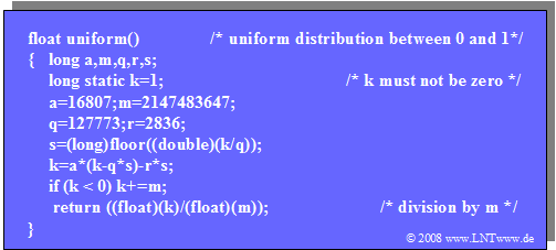
Multiplicative Congruental Generator (C program)

$\text{Example 2:}$ We analyze the "Multiplicative Congruental Generator" in more detail:

The algorithm, however, cannot be implemented directly on a 32–bit computer, since the multiplication result requires up to 46 bits.

But it can be modified in such a way that at no time during the calculation the 32–bit integer number range is exceeded.

The C program $\text{uniform( )}$ thus modified is given on the right.

Exercises for the chapter

Exercise 3.5: Triangular and Trapezoidal Signal

Exercise 3.5Z: Antenna Areas