Sampling of Analog Signals and Signal Reconstruction

Open Applet in new Tab   Deutsche Version Öffnen

Applet Description

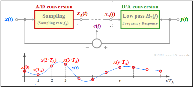
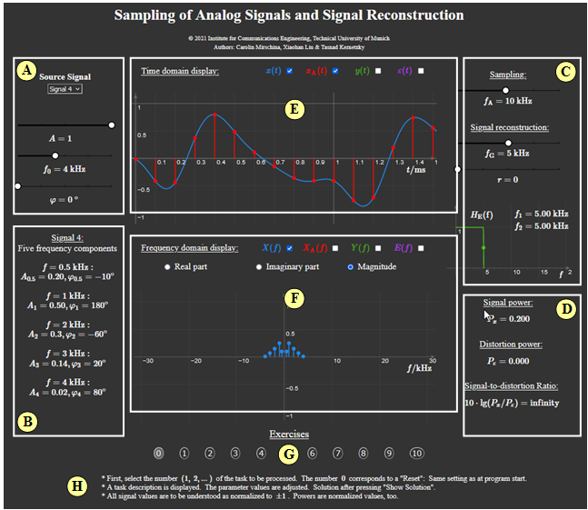
The applet deals with the system components  "sampling"  and  "signal reconstruction", two components that are of great importance for understanding the  "Puls code modulation"  $({\rm PCM})$  for example.   The upper graphic shows the model on which this applet is based.  Below it are the samples  $x(\nu \cdot T_{\rm A})$  of the time continuous signal  $x(t)$. The (infinite) sum over all these samples is called the sampled signal  $x_{\rm A}(t)$.

Top:    Underlying model for sampling and signal reconstruction
Bottom:   Example for time discretization of the continuous–time signal  $x(t)$

• At the transmitter, the time discrete (sampled) signal  $x_{\rm A}(t)$  is obtained from the continuous–time signal  $x(t)$.  This process is called  sampling   or  A/D conversion.
• The corresponding program parameter for the transmitter is the sampling rate  $f_{\rm A}= 1/T_{\rm A}$.  The lower graphic shows the sampling distance  $T_{\rm A}$ .
• In the receiver, the discrete-time received signal  $y_{\rm A}(t)$  is used to generate the continuous-time sink signal  $y(t)$    ⇒   signal reconstruction  or  D/A conversion  corresponding to the receiver frequency response  $H_{\rm E}(f)$.

The applet does not consider the PCM blocks  "Quantization"and  "encoding/decoding".   The digital transmission channel is assumed to be ideal. 

Receiver frequency response  $H_{\rm E}(f)$

The following consequences result from this:

• In the program simplifying  $y_{\rm A}(t) = x_{\rm A}(t)$  is set.
• With suitable system parameters, the error signal   $\varepsilon(t) = y(t)-x(t)\equiv 0$  is therefore also possible.

The sampling theorem and the signal reconstruction can be better explained in the frequency domain.  Therefore all spectral functions are displayed in the program;

             $X(f)\ \bullet\!\!-\!\!\!-\!\!\!-\!\!\circ\,\ x(t)$,  $X_{\rm A}(f)\ \bullet\!\!-\!\!\!-\!\!\!-\!\!\circ\,\ x_{\rm A}(t)$,  $Y(f)\ \bullet\!\!-\!\!\!-\!\!\!-\!\!\circ\,\ y(t)$,  $E(f)\ \bullet\!\!-\!\!\!-\!\!\!-\!\!\circ\,\ \varepsilon(t).$ 

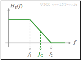
Parameters for the receiver frequency response  $H_{\rm E}(f)$  are the cut–off frequency and the rolloff factor  (see lower graph):

$$f_{\rm G} = \frac{f_2 +f_1}{2},\hspace{1cm}r = \frac{f_2 -f_1}{f_2 +f_1}.$$

Notes:

(1)   All signal values are normalized to  $\pm 1$.

(2)   The power calculation is done by integration over the respective period duration  $T_0$:

$$P_x = \frac{1}{T_0} \cdot \int_0^{T_0} x^2(t)\ {\rm d}t,\hspace{0.8cm}P_\varepsilon = \frac{1}{T_0} \cdot \int_0^{T_0} \varepsilon^2(t).$$

(3)   The signal power  $P_x$  and the distortion power  $P_\varepsilon$  are also output in normalized form, which implicitly assumes the reference resistance  $R = 1\, \rm \Omega$ ;

(4)   From these the signal–distortion–distance  $10 \cdot \lg \ (P_x/P_\varepsilon)$  can be calculated.

(5)   Does the spectral function  $X(f)$  for positive frequencies consists of  $I$  Dirac delta lines with the (possibly complex) weights  $X_1$, ... , $X_I$,
          so applies to the transmission power taking into account the mirror-image lines at the negative frequencies:

$$P_x = 2 \cdot \sum_{i=1}^I |X_k|^2.$$

(6)   Correspondingly, the following applies to the distortion power if the spectral function  $E(f)$  in the range  $f>0$  has  $J$  Dirac delta lines with weights  $E_1$, ... , $E_J$:

$$P_\varepsilon = 2 \cdot \sum_{j=1}^J |E_j|^2.$$

Theoretical Background

Description of sampling in the time domain

For the time discretization of the continuous-time signal  $x(t)$

In the following, we use the following nomenclature to describe the sampling:

• let the continuous-time signal be  $x(t)$.
• Let the time-discretized signal sampled at equidistant intervals  $T_{\rm A}$  be  $x_{\rm A}(t)$.
• Out of the sampling time points  $\nu \cdot T_{\rm A}$  always holds  $x_{\rm A}(t) \equiv 0$.
• The run variable  $\nu$  be an  "integer":     $\nu \in \mathbb{Z} = \{\hspace{0.05cm} \text{...}\hspace{0.05cm} , –3, –2, –1, \hspace{0.2cm}0, +1, +2, +3, \text{...} \hspace{0.05cm}\}$.
• In contrast, at the equidistant sampling times with the constant  $K$, the result is:

$$x_{\rm A}(\nu \cdot T_{\rm A}) = K \cdot x(\nu \cdot T_{\rm A})\hspace{0.05cm}.$$

The constant depends on the type of time discretization. For the above sketch $K = 1$ is valid.

Description of sampling with the Dirac delta pulse

In the following, we assume a slightly different form of description.  The following pages will show that these equations, which take some getting used to, do lead to useful results if they are applied consistently.

$\text{Definitions:}$ 

• By  sampling  we mean here the multiplication of the time-continuous signal  $x(t)$  by a  Dirac delta pulse:

$$x_{\rm A}(t) = x(t) \cdot p_{\delta}(t)\hspace{0.05cm}.$$

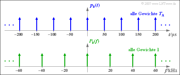
• The  Dirac delta pulse (in the time domain)  consists of infinitely many Dirac delta pulses, each equally spaced  $T_{\rm A}$  and all with equal pulse weight  $T_{\rm A}$:

$$p_{\delta}(t) = \sum_{\nu = - \infty }^{+\infty} T_{\rm A} \cdot \delta(t- \nu \cdot T_{\rm A} )\hspace{0.05cm}.$$

Based on this definition, the following properties result for the sampled signal:

$$x_{\rm A}(t) = \sum_{\nu = - \infty }^{+\infty} T_{\rm A} \cdot x(\nu \cdot T_{\rm A})\cdot \delta (t- \nu \cdot T_{\rm A} )\hspace{0.05cm}.$$

• The sampled signal at the considered time  $(\nu \cdot T_{\rm A})$  ist gleich  $T_{\rm A} \cdot x(\nu \cdot T_{\rm A}) · \delta (0)$.
• Since  $\delta (t)$  at time  $t = 0$  is infinite, actually all signal values  $x_{\rm A}(\nu \cdot T_{\rm A})$  are also infinite and also the factor  $K$ introduced above.
• Two samples  $x_{\rm A}(\nu_1 \cdot T_{\rm A})$  and  $x_{\rm A}(\nu_2 \cdot T_{\rm A})$  however, differ in the same proportion as the signal values  $x(\nu_1 \cdot T_{\rm A})$  and  $x(\nu_2 \cdot T_{\rm A})$.
• The samples of  $x(t)$  appear in the pulse weights of the Dirac delta functions:
• The additional multiplication by  $T_{\rm A}$  is necessary so that  $x(t)$  and  $x_{\rm A}(t)$  have the same unit.  Note here that  $\delta (t)$  itself has the unit "1/s".

Description of sampling in the frequency domain

The spectrum of the sampled signal  $x_{\rm A}(t)$  is obtained by applying the  "Convolution Theorem". This states that multiplication in the time domain corresponds to convolution in the spectral domain:

$$x_{\rm A}(t) = x(t) \cdot p_{\delta}(t)\hspace{0.2cm}\circ\!\!-\!\!\!-\!\!\!-\!\!\bullet\, \hspace{0.2cm} X_{\rm A}(f) = X(f) \star P_{\delta}(f)\hspace{0.05cm}.$$

If one develops the  Dirac delta pulse  $p_{\delta}(t)$   (in the time domain)   into a  "Fourier Series"  and transforms it using the  "Shifting Theorem"  into the frequency domain, the following correspondence   ⇒   "proof" results with the distance  $f_{\rm A} = 1/T_{\rm A}$  of two adjacent dirac delta lines in the frequency domain:

$$p_{\delta}(t) = \sum_{\nu = - \infty }^{+\infty} T_{\rm A} \cdot \delta(t- \nu \cdot T_{\rm A} )\hspace{0.2cm}\circ\!\!-\!\!\!-\!\!\!-\!\!\bullet\, \hspace{0.2cm} P_{\delta}(f) = \sum_{\mu = - \infty }^{+\infty} \delta (f- \mu \cdot f_{\rm A} ).$$

Dirac delta pulse in time and frequency domain with  $T_{\rm A} = 50\ {\rm µs}$  und  $f_{\rm A} = 1/T_{\rm A} = 20\ \text{kHz}$

The result states:

• The Dirac delta pulse  $p_{\delta}(t)$  in the time domain consists of infinitely many Dirac delta pulses, each at the same distance  $T_{\rm A}$  and all with the same pulse weight  $T_{\rm A}$.
• The Fourier transform of  $p_{\delta}(t)$  again gives a Dirac delta pulse, but now in the frequency domain   ⇒   $P_{\delta}(f)$.
• Also  $P_{\delta}(f)$  consists of infinitely many Dirac delta pulses, now in the respective spacing  $f_{\rm A} = 1/T_{\rm A}$  and all with pulse weight  $1$.
• The distances of the Dirac delta lines in time and frequency domain thus follow the  "Reciprocity Theorem":   $T_{\rm A} \cdot f_{\rm A} = 1 \hspace{0.05cm}.$

From this follows:   From the spectrum  $X(f)$  is obtained by convolution with the Dirac delta line shifted by  $\mu \cdot f_{\rm A}$ :

$$X(f) \star \delta (f- \mu \cdot f_{\rm A} )= X (f- \mu \cdot f_{\rm A} )\hspace{0.05cm}.$$

Applying this result to all Dirac delta lines of the Dirac delta pulse, we finally obtain:

$$X_{\rm A}(f) = X(f) \star \sum_{\mu = - \infty }^{+\infty} \delta (f- \mu \cdot f_{\rm A} ) = \sum_{\mu = - \infty }^{+\infty} X (f- \mu \cdot f_{\rm A} )\hspace{0.05cm}.$$

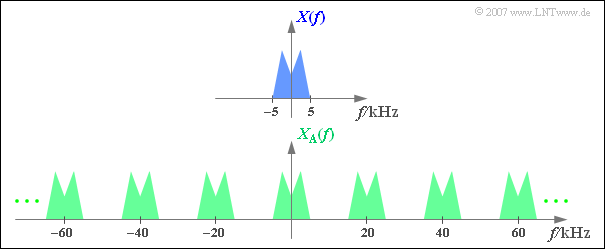
$\text{Conclusion:}$  Sampling the analog time signal  $x(t)$  at equidistant intervals  $T_{\rm A}$  results in the spectral domain in a  periodic continuation  of  $X(f)$  with frequency spacing  $f_{\rm A} = 1/T_{\rm A}$.

Spectrum of the sampled signal

$\text{Example 1:}$  The upper graph shows  (schematic!)  the spectrum  $X(f)$  of an analog signal  $x(t)$, which contains frequencies up to  $5 \text{ kHz}$ .

Sampling the signal at the sampling rate  $f_{\rm A}\,\text{ = 20 kHz}$, i.e., at the respective spacing  $T_{\rm A}\, = {\rm 50 \, µs}$  yields the periodic spectrum  $X_{\rm A}(f)$ sketched below.

• Since the Dirac delta functions are infinitely narrow, the sampled signal  $x_{\rm A}(t)$  also contains arbitrary high frequency components.
• Correspondingly, the spectral function  $X_{\rm A}(f)$  of the sampled signal is extended to infinity.

Signal reconstruction

Joint model of "signal sampling" and "signal reconstruction"

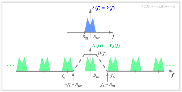
Signal sampling is not an end in itself in a digital transmission system, but it must be reversed at some point  For example, consider the following system:

• The analog signal  $x(t)$  with bandwidth  $B_{\rm NF}$  is sampled as described above.
• At the output of an ideal transmission system, the also discrete-time signal  $y_{\rm A}(t) = x_{\rm A}(t)$  is present.
• The question now is how the block   signal reconstruction   has to be designed so that also  $y(t) = x(t)$  holds.

Frequency domain representation of the "signal reconstruction"

The solution is simple if you look at the spectral functions:  

One obtains from  $Y_{\rm A}(f)$  the spectrum  $Y(f) = X(f)$  by a low-pass filter with the  "Frequency response"  $H_{\rm E}(f)$, which 

• passes the low frequencies unaltered:

$$H_{\rm E}(f) = 1 \hspace{0.3cm}{\rm{for}} \hspace{0.3cm} |f| \le B_{\rm NF}\hspace{0.05cm},$$

• completely suppresses the high frequencies:

$$H_{\rm E}(f) = 0 \hspace{0.3cm}{\rm{for}} \hspace{0.3cm} |f| \ge f_{\rm A} - B_{\rm NF}\hspace{0.05cm}.$$

Further, it can be seen from the accompanying graph:   As long as the above two conditions are satisfied,  $H_{\rm E}(f)$  can be arbitrarily shaped in the range from  $B_{\rm NF}$  to  $f_{\rm A}-B_{\rm NF}$  ,

• for example linearly descending (dashed line)
• or also rectangular.

The Sampling Theorem

The complete reconstruction of the analog signal  $y(t)$  from the sampled signal  $y_{\rm A}(t) = x_{\rm A}(t)$  is only possible if the sampling rate  $f_{\rm A}$  corresponding to the bandwidth  $B_{\rm NF}$  of the message signal has been chosen correctly.

From the above graph, it can be seen that the following condition must be satisfied:   $f_{\rm A} - B_{\rm NF} > B_{\rm NF} \hspace{0.3cm}\Rightarrow \hspace{0.3cm}f_{\rm A} > 2 \cdot B_{\rm NF}\hspace{0.05cm}.$

$\text{Sampling theorem:}$  If an analog signal  $x(t)$  has only spectral components in the range  $\vert f \vert < B_{\rm NF}$, it can be completely reconstructed from its sampled signal  $x_{\rm A}(t)$  only if the sampling rate is sufficiently large:

$$f_{\rm A} ≥ 2 \cdot B_{\rm NF}.$$

Accordingly, the following must apply to the distance between two samples:

$$T_{\rm A} \le \frac{1}{ 2 \cdot B_{\rm NF} }\hspace{0.05cm}.$$

If the largest possible value   ⇒   $T_{\rm A} = 1/(2B_{\rm NF})$  is used for sampling,

• so, for signal reconstruction of the analog signal from its samples.
• an ideal, rectangular low-pass filter with cut off frequency  $f_{\rm G} = f_{\rm A}/2 = 1/(2T_{\rm A})$  must be used.

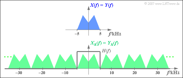
$\text{Example 2:}$  The graph shows above the spectrum  $\pm\text{ 5 kHz}$  of an analog signal limited to  $X(f)$  below the spectrum  $X_{\rm A}(f)$  of the signal sampled at distance  $T_{\rm A} =\,\text{ 100 µs}$  ⇒   $f_{\rm A}=\,\text{ 10 kHz}$.

Sampling theorem in the frequency domain

Additionally drawn is the frequency response  $H_{\rm E}(f)$  of the low-pass receiving filter for signal reconstruction, whose cutoff frequency must be exactly  $f_{\rm G} = f_{\rm A}/2 = 5\,\text{ kHz}$ .

• With any other  $f_{\rm G}$ value, there would be  $Y(f) \neq X(f)$.
• For  $f_{\rm G} < 5\,\text{ kHz}$  the upper  $X(f)$ portions are missing.
• At  $f_{\rm G} > 5\,\text{ kHz}$  there are unwanted spectral components in  $Y(f)$ due to convolution products.

If at the transmitter the sampling had been done with a sampling rate  $f_{\rm A} < 10\,\text{ kHz}$    ⇒   $T_{\rm A} >100 \ {\rm µ s}$, the analog signal  $y(t) = x(t)$  would not be reconstructible from the samples  $y_{\rm A}(t)$  in any case.

Exercises

• First, select the number  $(1,\ 2, \text{...} \ )$  of the task to be processed.  The number  $0$  corresponds to a "Reset":  Same setting as at program start.
• A task description is displayed.  The parameter values are adjusted.  Solution after pressing "Show Solution".
• All signal values are to be understood as normalized to  $\pm 1$.  Powers are normalized values, too.

(1)  Source signal:  $x(t) = A \cdot \cos (2\pi \cdot f_0 \cdot t -\varphi)$  with  $f_0 = \text{4 kHz}$.   Sampling with  $f_{\rm A} = \text{10 kHz}$.  Rectanglular low-pass;  cut off frequency:  $f_{\rm G} = \text{5 kHz}$.
            Interpret the shown graphics and evaluate the present signal reconstruction for all permitted parameter values of $A$  and $\varphi$.

•  The spectrum  $X(f)$  consists of two Dirac functions at  $\pm \text{4 kHz}$, each with impulse weight  $0.5$.
•  By the periodic continuation  $X_{\rm A}(f)$  has lines of equal height at  $\pm \text{4 kHz}$,  $\pm \text{6 kHz}$,  $\pm \text{14 kHz}$,  $\pm \text{16 kHz}$,  $\pm \text{24 kHz}$,  $\pm \text{26 kHz}$,  etc.
•  The rectangular low-pass with the cut off frequency  $f_{\rm G} = \text{5 kHz}$  removes all lines except the two at  $\pm \text{4 kHz}$  ⇒  $Y(f) =X(f)$  ⇒  $y(t) =x(t)$  ⇒   $P_\varepsilon = 0$.
•  The signal reconstruction works here perfectly  $(P_\varepsilon = 0)$  for all amplitudes $A$  and any phases $\varphi$.

(2)  Continue with  $A=1$,  $f_0 = \text{4 kHz}$,  $\varphi=0$,  $f_{\rm A} = \text{10 kHz}$,  $f_{\rm G} = \text{5 kHz}$.   What is the influence of the rolloff–factors  $r=0.2$,  $r=0.5$  and   $r=1$?
          Specify the power values  $P_x$  and  $P_\varepsilon$ .   For which  $r$–values is  $P_\varepsilon= 0$?  Do these results also apply to other  $A$  and  $\varphi$?

•  With  $|X(f = \pm \text{4 kHz})|=0.5$  the signal power is  $P_x = 2\cdot 0.5^2 = 0.5$.  The distortion power  $P_\varepsilon$  depends significantly on the rolloff–factor  $r$ .
•  $P_\varepsilon$  is zero for  $r \le 0.2$.  Then the  $X_{\rm A}(f)$ line at  $f_0 = \text{4 kHz}$  is not changed by the low-pass and the unwanted  line at  $\text{6 kHz}$  is fully suppressed.
•  $r = 0.5$ :  $Y(f = \text{4 kHz}) = 0.35$,  $Y(f = \text{6 kHz}) = 0.15$  ⇒   $|E(f = \text{4 kHz})| = |E(f = \text{6 kHz})|= 0. 15$  ⇒  $P_\varepsilon = 0.09$  ⇒  $10 \cdot \lg \ (P_x/P_\varepsilon)=7.45\ \rm dB$.
• $r = 1.0$ :  $Y(f = \text{4 kHz}) = 0.3$,  $Y(f = \text{6 kHz}) = 0.2$  ⇒   $|E(f = \text{4 kHz})| = |E(f = \text{6 kHz})|= 0. 2$  ⇒  $P_\varepsilon = 0.16$  ⇒  $10 \cdot \lg \ (P_x/P_\varepsilon)=4.95\ \rm dB$.
•  For all  $r$  the distortion power $P_\varepsilon$  is independent of  $\varphi$.   The amplitude  $A$  affects  $P_x$  and  $P_\varepsilon$  in the same way   ⇒   the quotient is independent of  $A$.

(3)  Now apply  $A=1$,  $f_0 = \text{5 kHz}$,  $\varphi=0$,  $f_{\rm A} = \text{10 kHz}$,  $f_{\rm G} = \text{5 kHz}$,  $r=0$  $($rectangular low–pass$)$.   Interpret the result of the signal reconstruction.

•   $X(f)$  consists of two Dirac delta lines at  $\pm \text{5 kHz}$  $($weight  $0.5)$.  By periodic continuation  $X_{\rm A}(f)$  has lines at  $\pm \text{5 kHz}$,  $\pm \text{15 kHz}$,  $\pm \text{25 kHz}$,  etc.
•   The  rectanglular low-pass  removes the lines at  $\pm \text{15 kHz}$,  $\pm \text{25 kHz}$.  The lines at  $\pm \text{5 kHz}$  are halved because of  $H_{\rm E}(\pm f_{\rm G}) = H_{\rm E}(\pm \text{5 kHz}) = 0.5$.
•    ⇒   $\text{Weights of }X(f = \pm \text{5 kHz})$:  $0.5$   #   $\text{Weights of }X(f_{\rm A} = \pm \text{5 kHz})$:  $1. 0$;     #   $\text{Weights of }Y(f = \pm \text{5 kHz})$:  $0.5$   ⇒   $Y(f)=X(f)$.
•  So the signal reconstruction works perfectly here too  $(P_\varepsilon = 0)$.  The same is true for the phase  $\varphi=180^\circ$   ⇒   $x(t) = -A \cdot \cos (2\pi \cdot f_0 \cdot t)$.

(4)  The settings of  $(3)$  continue to apply except for  $\varphi=30^\circ$.  Interpret the differences from the setting  $(3)$   ⇒   $\varphi=0^\circ$.

•  Phase relations are lost.  The sink signal  $y(t)$  is cosine-shaped  $(\varphi_y=0^\circ)$  with by the factor  $\cos(\varphi_x)$  smaller amplitude than the source signal  $x(t)$.
•  Justification in the frequency domain:  In the periodic continuation of  $X(f)$  ⇒  $X_{\rm A}(f)$  only the real parts are to be added.  The imaginary parts cancel out.
•  The Dirac delta line of  $X(f)$  at frequency  $f_0$   ⇒   $X(f_0)$  is complex,   $Y(f_0)$  is real, and  $E(f_0)$  is imaginary   ⇒   $\varepsilon(t)$  is minus–sinusoidal   ⇒   $P_\varepsilon = 0. 125$.

(5)  Illustrate again the result of  $(4)$  compared to the settings  $f_0 = \text{5 kHz}$,  $\varphi=30^\circ$,  $f_{\rm A} = \text{11 kHz}$,  $f_{\rm G} = \text{5.5 kHz}$.

•  With this setting, the spectrum  $X_{\rm A}(f)$  also has a positive imaginary part at  $\text{5 kHz}$  and a negative imaginary part of the same magnitude at  $\text{6 kHz}$.
•  The rectangular low-pass with cutoff frequency  $\text{5.5 kHz}$  removes this second component.  Thus, with the new setting  $Y(f) =X(f)$   ⇒   $P_\varepsilon = 0$.
•  Any $f_0$ oscillation of arbitrary phase is error-free reconstructible from its samples if  $f_{\rm A} = 2 \cdot f_{\rm 0} + \mu, \ f_{\rm G}= f_{\rm A}/2$  $($any small $\mu>0)$.
•  For value–continuous spectrum with   $X(|f|> f_0) \equiv 0$  ⇒   $\big[$no diraclines at $\pm f_0 \big ]$  the sampling rate  $f_{\rm A} = 2 \cdot f_{\rm 0}$  is sufficient in principle.

(5)  Verdeutlichen Sie sich nochmals das Ergebnis von  (4)  im Vergleich zu den Einstellungen  $f_0 = \text{5 kHz}$,  $\varphi=30^\circ$,  $f_{\rm A} = \text{11 kHz}$,  $f_{\rm G} = \text{5.5 kHz}$.

•  Bei dieser Einstellung hat das  $X_{\rm A}(f)$–Spektrum auch einen positiven Imaginärteil bei  $\text{5 kHz}$  und einen negativen Imaginärteil gleicher Höhe bei  $\text{6 kHz}$.
•  Der Rechteck–Tiefpass mit der Grenzfrequenz  $\text{5.5 kHz}$  entfernt diesen zweiten Anteil.  Somit ist bei dieser Einstellung  $Y(f) =X(f)$   ⇒   $P_\varepsilon = 0$.
•  Jede  $f_0$–Schwingung beliebiger Phase ist fehlerfrei aus seinen Abtastwerten rekonstruierbar, falls  $f_{\rm A} = 2 \cdot f_{\rm 0} + \mu, \ f_{\rm G}= f_{\rm A}/2$  $($beliebig kleines $\mu>0)$.
•  Bei wertkontinuierlichem Spektrum mit   $X(|f|> f_0) \equiv 0$  ⇒   $\big[$keine Diraclinien bei $\pm f_0 \big ]$ genügt grundsätzlich die Abtastrate  $f_{\rm A} = 2 \cdot f_{\rm 0}$.

(6)  The settings of  $(3)$  and  $(4)$  continue to apply except for  $\varphi=90^\circ$.  Interpret the plots in the time and frequency domain.

•  The source signal is sampled exactly at its zero crossings   ⇒   $x_{\rm A}(t) \equiv 0$   ⇒     $y(t) \equiv 0$   ⇒   $\varepsilon(t)=-x(t)$   ⇒   $P_\varepsilon = P_x$   ⇒   $10 \cdot \lg \ (P_x/P_\varepsilon)=0\ \rm dB$.
•  Description in the frequency domain:   As in  $(4)$  the imaginary parts of  $X_{\rm A}(f)$  cancel out.  Also the real parts of  $X_{\rm A}(f)$  are zero because of the sinusoid.

(7)  Now consider the  $\text {Source Signal 2}$.  Let the other parameters be  $f_{\rm A} = \text{5 kHz}$,  $f_{\rm G} = \text{2.5 kHz}$,  $r=0$.  Interpret the results.

•  The source signal has spectral components up to  $\pm \text{2 kHz}$.  The signal power is $P_x = 2 \cdot \big[0.1^2 + 0.25^2+0.15^2\big]= 0.19$. 
•  With the sampling rate  $f_{\rm A} = \text{5 kHz}$  and the receiver parameters  $f_{\rm G} = \text{2.5 kHz}$  and  $r=0$, the signal reconstruction works perfectly:  $P_\varepsilon = 0$.
•  Likewise with the trapezoidal low–pass with  $f_{\rm G} = \text{2.5 kHz}$, if for the rolloff factor holds:  $r \le 0.2$.

(8)  What happens if the cutoff frequency  $f_{\rm G} = \text{1.5 kHz}$  of the rectangular low–pass filter is too small?  In particular, interpret the error signal  $\varepsilon(t)=y(t)-x(t)$.

•  The error signal  $\varepsilon(t)=-0.3 \cdot \cos(2\pi \cdot \text{2 kHz} \cdot t -60^\circ)=0. 3 \cdot \cos(2\pi \cdot \text{2 kHz} \cdot t +120^\circ)$  is equal to the (negated) signal component at  $\text{2 kHz}$. 
•  The distortion power is  $P_\varepsilon=2 \cdot 0.15^2= 0.045$  and the signal–to–distortion ratio  $10 \cdot \lg \ (P_x/P_\varepsilon)=10 \cdot \lg \ (0.19/0.045)= 6.26\ \rm dB$.

(9)  What happens if the cutoff frequency  $f_{\rm G} = \text{3.5 kHz}$  of the rectangular low–pass filter is too large?  In particular, interpret the error signal  $\varepsilon(t)=y(t)-x(t)$.

•  The error signal  $\varepsilon(t)=0.3 \cdot \cos(2\pi \cdot \text{3 kHz} \cdot t +60^\circ)$  is now equal to the  $\text{3 kHz}$  portion of the sink signal  $y(t)$  not removed by the low-pass filter.
•  Compared to the subtask  $(8)$  the frequency changes from  $\text{2 kHz}$  to  $\text{3 kHz}$  and also the phase relationship.
•  The amplitude of this  $\text{3 kHz}$ error signal is equal to the amplitude of the  $\text{2 kHz}$ portion of  $x(t)$.  Again  $P_\varepsilon= 0.045$,  $10 \cdot \lg \ (P_x/P_\varepsilon)= 6.26\ \rm dB$.

(10)  Finally, we consider the  $\text {source signal 4}$  $($portions until  $\pm \text{4 kHz})$, as well as  $f_{\rm A} = \text{5 kHz}$,  $f_{\rm G} = \text{2. 5 kHz}$,  $0 \le r\le 1$.  Interpretation of results.

•  Up to  $r=0.2$  the signal reconstruction works perfectly  $(P_\varepsilon = 0)$.  If one increases  $r$, then  $P_\varepsilon$  increases continuously and  $10 \cdot \lg \ (P_x/P_\varepsilon)$  decreases.
•  With  $r=1$  the signal frequencies  $\text{0.5 kHz}$,  ...,  $\text{4 kHz}$  are attenuated, the more the higher the frequency is,  for example  $H_{\rm E}(f=\text{4 kHz}) = 0.6$.
•  Similarly,  $Y(f)$  also includes components at frequencies  $\text{6 kHz}$,  $\text{7 kHz}$,  $\text{8 kHz}$,  $\text{9 kHz}$  and  $\text{9.5 kHz}$ due to periodic continuation.
•  At the sampling times  $t\hspace{0.05cm}' = n \cdot T_{\rm A}$, the signals  $x(t\hspace{0.05cm}')$  and  $y(t\hspace{0.05cm}')$  agree exactly  ⇒   $\varepsilon(t\hspace{0.05cm}') = 0$.  In between, not  ⇒   small distortion power   $P_\varepsilon = 0.008$.

Applet Manual

Screenshot Korrektur

    (A)     Selection:   Encoding
               (binary,  quaternary,  AMI–code,  duobinary code).

    (B)     Selection:   Detection base pulse
                (by Gaussian–LP,  CRO–Nyquist,  by slit–LP}

    (C)     Parameter input to  (B)
                 (cutoff frequency,  rolloff–factor,  rectangular wave duration)

    (D)     Eye diagram display control
                 (start,  pause/continue,  single step,  total,  reset).

    (E)     Velocity of the eye diagram representation.

    (F)     Representation:  Detection ground momentum  $g_d(t)$

    (G)     Representation:  detection useful signal  $d_{\rm S}(t - \nu \cdot T)$

    (H)     Representation:  Eye diagram in the range  $\pm T$

    ( I )'     Numerical output:  $ö_{\rm norm}$  (normalized eye opening).

    (J)'     Parameter input  $10 \cdot \lg \ E_{\rm B}/N_0$  for  (K)

    (K)'     Numeric output:  $\sigma_{\rm norm}$  (normalized noise rms).

    (L)'     Numeric output:  $p_{\rm U}$  (worst case error probability)

    (M)'     Range for experimental performance:   Task selection.

    (N)'     Range for the execution of experiments:   Task selection

    (O)'     Range for carrying out the experiment:   Show sample solution

About the Authors

This interactive calculation tool was designed and implemented at the  Institute for Communications Engineering  at the  Technical University of Munich.

• The first version was created in 2008 by Slim Lamine  as part of his diploma thesis with “FlashMX – Actionscript” (Supervisor: Günter Söder).

• Last revision and English version 2020/2021 by  Carolin Mirschina  in the context of a working student activity. 

The conversion of this applet to HTML 5 was financially supported by  Studienzuschüsse  ("study grants")  of the TUM Faculty EI.  We thank.

Once again:  Open Applet in new Tab

Open Applet in new Tab   Deutsche Version Öffnen