Contents
Channel model and Rice PDF
The Rayleigh distribution describes the mobile communication channel under the assumption that there is no direct path and thus the multiplicative factor $z(t) = x(t) + {\rm j} \cdot y(t)$ is solely composed of diffusely scattered components.
If a direct component ( Line of Sight, $\rm LoS)$ is present, it is necessary to add direct components $x_0$ and/or $y_0$ to the zero mean Gaussian processes $x(t)$ and $y(t)$:
- \[x(t) \hspace{0.1cm} \Rightarrow \hspace{0.1cm} x(t) +x_0 \hspace{0.05cm}, \hspace{0.2cm} y(t) \hspace{0.1cm} \Rightarrow \hspace{0.1cm} y(t) +y_0\hspace{0.05cm},\]
- \[z(t) = x(t) + {\rm j} \cdot y(t) \hspace{0.1cm} \Rightarrow \hspace{0.1cm} z(t) +z_0 \hspace{0.05cm},\hspace{0.2cm} z_0 = x_0 + {\rm j} \cdot y_0\hspace{0.05cm}.\]
The graphic shows this Rice fading channel model. As a special case, the Rayleigh model results when $x_0 = y_0= 0$ .
The Rice fading model can be summarized as follows, see also [Hin08][1]:
- The real part $x(t)$ is gaussian distributed with mean value $x_0$ and variance $\sigma ^2$.
- The imaginary part $y(t)$ is also gaussian distributed $($mean $y_0$, equal variance $\sigma ^2)$ and independent of $x(t)$.
- For $z_0 \ne 0$ the value $|z(t)|$ is riceversified, from which the term „Rice–Fading” is derived.
- To simplify the notation we set $|z(t)| = a(t)$. For $a < 0$ it's PDF is $f_a(a) \equiv 0$, for $a \ge 0$ the following equation applies, where $\rm I_0(\cdot)$ denotes the modified Bessel–function of zero order:
- \[f_a(a) = \frac{a}{\sigma^2} \cdot {\rm exp} \big [ -\frac{a^2 + |z_0|^2}{2\sigma^2}\big ] \cdot {\rm I}_0 \left [ \frac{a \cdot |z_0|}{\sigma^2} \right ]\hspace{0.5cm}\text{mit}\hspace{0.5cm}{\rm I }_0 (u) = {\rm J }_0 ({\rm j} \cdot u) = \sum_{k = 0}^{\infty} \frac{ (u/2)^{2k}}{k! \cdot \Gamma (k+1)} \hspace{0.05cm}.\]
- The greater the „direct path power” $(|z_0|^2)$ compared to the power of the stray components $(2\sigma^2)$ the better suited for digital signal transmission is the mobile communication channel
- If $|z_0| \gg \sigma$ $($factor $3$ or more$)$, the Rice–PDF can be approximated accurately by a Gaussian distribution with mean $|z_0|$ and variance $\sigma$
- In contrast to Rayleigh fading ⇒ $z_0 \equiv 0$, the phase at Rice fading is not equally distributed, but there is a preferred direction $\phi_0 = \arctan(y_0/x_0)$. Often one sets $y_0 = 0$ ⇒ $\phi_0 = 0$.
Example of signal behaviour with Rice fading
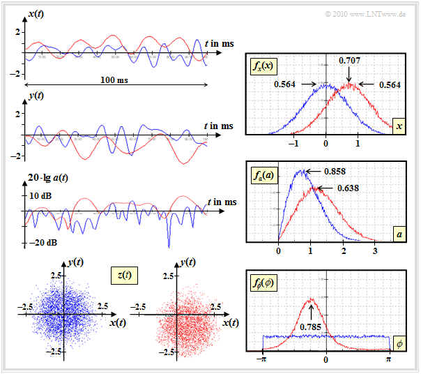
The diagram shows typical signal characteristics and density functions of two mobile communication channels:
- Rayleigh fading (blue curves) with
- $${\rm E}\big [|z(t))|^2\big ] = 2 \cdot \sigma^2 = 1,$$
- Rice fading (red curves) with the same $\sigma$ and 
- $$x_0 = 0.707,\ \ y_0 = -0.707.$$
For the generation of the signal sections according to the above model, the maximum Doppler frequency $f_\text{D, max} = 100 \ \rm Hz$ was used as reference.
The autocorrelation function $\rm (ACF)$ and power density spectrum $\rm (PSD)$ of Rayleigh and Rice differ only slightly, other than adjusted parameter values. The following applies:
- \[\varphi_z ({\rm \Delta}t)\Bigg |_{\hspace{0.1cm}{\rm Rice}} \hspace{-0.5cm} = \varphi_z ({\rm \Delta}t)\Bigg |_{\hspace{0.1cm}{\rm Rayleigh}} \hspace{-0.8cm} + |z_0|^2 \hspace{0.05cm},\]
- \[ {\it \Phi}_z(f_{\rm D})\Bigg |_{\hspace{0.1cm}{\rm Rice}} \hspace{-0.5cm} = {\it \Phi}_z(f_{\rm D})\Bigg |_{\hspace{0.1cm}{\rm Rayleigh}} \hspace{-0.8cm} + |z_0|^2 \cdot \delta (f_{\rm D}) \hspace{0.05cm}.\]
It is taken into account that the spectral representation of a DC component leads to a Dirac function.
It should be noted about this graphic:
- The real parts $x(t)$ of Rayleigh (blue) and Rice (red) only differ by the constant $x_0 = 0.707$. The statistical properties are otherwise the same: Gaussian PDF $f_x(x)$ with variance $\sigma = 0.707$, either zero-mean (Rayleigh) or with mean $x_0$ (Rice).
- In the imaginary part $y(t)$ of the Rice distribution one can additionally recognize the direct component $y_0 = -0.707$. The (here not shown) PDF $f_y(y)$ is thus a Gaussian curve with the variance $\sigma = 0. 707$ around the mean value $ y_0 = -0.707$, thus axisymmetrical to the shown PDF $f_x(x)$.
- The (logarithmic) representation of ⇒ $a(t) =|z(t)|$ shows that the red curve is usually above the blue one. This can also be read from the PDF $f_a(a)$ .
- For the Rice channel, the error probability is lower than for Rayleigh when AWGN is taken into account, since the receiver gets a lot of usable energy via the Rice direct path.
- The PDF $f_\phi(\phi)$ shows the preferred angle $\phi \approx 45^\circ$ of the given Rice channel The complex factor $z(t)$ is located mainly in the fourth quadrant because of $x_0 > 0$ and $y_0 < 0$ , whereas in the Rayleigh channel all quadrants are equally probable.
Exercises to the chapter
Exercise 1.6: Autocorrelation Function and PSD with Rice Fading
Exercise 1.6Z: Comparison of Rayleigh and Rice
Exercise 1.7: PDF of Rice Fading
List of sources
- ↑ Hindelang, T.: Mobile Communications. Vorlesungsmanuskript. Lehrstuhl für Nachrichtentechnik, TU München, 2008.

