Probability Density Function (PDF)

# OVERVIEW OF THE THIRD MAIN CHAPTER #

We consider here continuous random variables, i.e., random variables which can assume infinitely many different values, at least in certain ranges of values.

Their applications in information and communication technology are manifold;
They are used, among other things, for the simulation of noise signals and for the description of fading effects.

We restrict ourselves at first to the statistical description of the amplitude distribution. Inner statistical bindings of the underlying processes are considered only in the following main chapters 4 and 5.

In detail, the following are treated:

the relationship between probability density function and cumulative distribution function;
the calculation of expected values and moments;
some special cases: uniform distribution, Gaussian distribution, exponential distribution, Laplace distribution, Rayleigh distribution, Rice distribution, Cauchy distribution;
the generation of continuous random variables on a computer.

The first section "Probability Density Function" is organized as follows:

Properties of continuous random variables

In the second chapter it was shown that the amplitude distribution of a discrete random variable is completely determined by its $M$ occurrence probabilities, where the step number $M$ usually has a finite value.

Now we consider continuous (value) random variables. By this we mean random variables whose possible numerical values are uncountable ⇒ $M \to \infty$.

Further it shall hold:

In the following we denote continuous random variables (mostly) with $x$ in contrast to the discrete random variables, which are denoted with $z$ as before.
No statement is made here about a possible time discretization, i.e., continuous random variables can be discrete in time.
Further, we assume for this chapter that there are no statistical bindings between the individual samples $x_ν$, or at least leave them out of consideration.

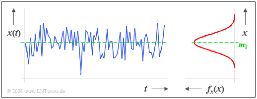
The following image shows a section of a stochastic noise signal $x(t)$ whose instantaneous value can be taken as a continuous random variable $x$.

Signal and PDF of a Gaussian noise signal

From the probability density function (PDF) shown on the right, it can be seen that instantaneous values around the mean $m_1$ occur most frequently for this example signal. Since there are no statistical bindings between the samples $x_ν$, such a signal is also referred to as white noise.

Definition of the probability density function

For a continuous random variable, the probabilities that it takes on quite specific values are equal to (wie übersetzt man 'identisch 0' besser?) $0$. Therefore, to describe a continuous random variable, we must always refer to the probability density function - abbreviated PDF.

The value of the probability density function $f_{x}(x)$ at location $x_\mu$ is equal to the probability that the instantaneous value of the random variable $x$ lies in an (infinitesimally small) interval of width $Δx$ around $x_\mu$ divided by $Δx$: $$f_x(x=x_\mu) = \lim_{\rm \Delta \it x \hspace{0.05cm}\to \hspace{0.05cm}\rm 0}\frac{\rm Pr \{\it x_\mu-\rm \Delta \it x/\rm 2 \le \it x \le x_\mu \rm +\rm \Delta \it x/\rm 2\}}{\rm \Delta \it x}.$$

This extremely important descriptive variable has the following properties:

Although it can be seen from the time course on the last subchapter that the most frequent signal components are at $x = m_1$ and the probability density function has its largest value here, the probability ${\rm Pr}(x = m_1$) that the instantaneous value is exactly equal to the mean $m_1$ is identical $0$.
For the probability that the random variable lies in the range between $x_u$ and $x_o$:

$${\rm Pr}(x_{\rm u} \le x \le x_{\rm o}) = \int_{x_{\rm u}}^{x_{\rm o}} f_{x}(x) \,{\rm d}x.$$

As an important normalization property, this yields for the area under the PDF with the boundary transitions $x_{\rm u} → \hspace{0.05cm} - \hspace{0.05cm} ∞$ and $x_{\rm o} → +∞:$

$$\int_{-\infty}^{+\infty} f_{x}(x) \,{\rm d}x = \rm 1.$$

The corresponding equation for discrete-value, $M$-level random variables states that the sum over the $M$ occurrence probabilities gives the value $1$.

Note on nomenclature: In the literature, we usually distinguish between the random variable $X$ and its realizations $x ∈ X$. Thus, the above definition equation is $$f_{X}(X=x) = \lim_{{\rm \Delta} x \hspace{0.05cm}\to \hspace{0.05cm} 0}\frac{{\rm Pr} \{ x-{\rm \Delta} x/2 \le X \le x +{\rm \Delta} x/ 2\}}{{\rm \Delta} x}.$$

We have largely dispensed with this more precise nomenclature in our learning tutorial so as not to use up two letters for one variable. Lowercase letters (like $x$) often denote signals and uppercase letters (like $X$) denote the associated spectra in our case. Nevertheless, today (2017) we honestly have to admit that the decision of 2001 was not quite fortunate.

PDF definition for discrete random variables

For reasons of a uniform representation of all random variables (both discrete-value and continuous-value), it is convenient to define the probability density function also for discrete random variables. Applying the definition equation of the last subchapter to discrete random variables, the PDF takes infinitely large values at some points $x_\mu$ due to the nonvanishingly small probability value and the limit transition $Δx → 0$. Thus, the PDF results in a sum of Dirac functions (resp. distributions): $$f_{x}(x)=\sum_{\mu=1}^{M}p_\mu\cdot {\rm \delta}( x-x_\mu).$$

The weights of these Dirac functions are equal to the probabilities $p_\mu = {\rm Pr}(x = x_\mu$).

Here is another note to help classify the different descriptive quantities for discrete and continuous random variables: Probability and probability density function are related in a similar way as in the book Signal Representation

a discrete spectral component of a harmonic oscillation ⇒ line spectrum, and
a continuous spectrum of an energy-limited (pulse-shaped) signal.

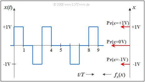
Below is a section of a rectangular signal with three possible values, where the signal value $0 \ \rm V$ occurs twice as often as the outer signal values ($\pm 1 \ \rm V$).

Thus, the corresponding PDF (proportions from top to bottom) is: $$f_{x}(x) = 0.25 \cdot \delta(x-{\rm 1 \rm V}) + 0.5\cdot \delta(x) + 0.25\cdot \delta (x + 1\rm V).$$

For a more in-depth look at the topic covered here, we recommend the following educational video:

Wahrscheinlichkeit und Wahrscheinlichkeitsdichtefunktion

Numerische Ermittlung der WDF

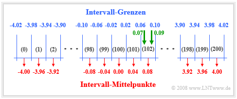
Sie sehen hier ein Schema zur numerischen Ermittlung der Wahrscheinlichkeitsdichtefunktion.

Setzt man voraus, dass die vorliegende Zufallsgröße $x$ außerhalb des Bereichs von $x_{\rm min} = –4.02$ bis $x_{\rm max} = +4.02$ nur vernachlässigbar kleine Anteile besitzt, so geht man folgendermaßen vor:

Man teilt den Wertebereich von $x$ in $I$ Intervalle gleicher Breite $Δx$ ein und definiert ein Feld $\text{WDF}[0 : I–1]$. In obiger Skizze ist $I = 201$ und dementsprechend $Δx = 0.04$ gewählt.
Die Zufallsgröße $x$ wird nun $N$ mal nacheinander aufgerufen und dabei jeweils geprüft, zu welchem Intervall $i_{\rm akt}$ die aktuelle Zufallsgröße $x_{\rm akt}$ gehört: $i_{\rm akt} = ({\rm int})((x + x_{\rm max})/Δx)$.
Das entsprechende Feldelement WDF( $i_{\rm akt}$) wird dann um $1$ erhöht. Nach $N$ Durchläufen beinhaltet dann $\text{WDF}[i_{\rm akt}]$ die Anzahl der Zufallszahlen, die zum Intervall $i_{\rm akt}$ gehören.
Die tatsächlichen WDF-Werte erhält man, wenn am Ende noch alle Feldelemente $\text{WDF}[i]$ mit $0 ≤ i ≤ I–1$ durch $N · Δx$ dividiert werden.

Aus den eingezeichneten grünen Pfeilen in obiger Grafik erkennt man:

Der Wert $x_{\rm akt} = 0.07$ führt zum Ergebnis $i_{\rm akt} =$ (int) ((0.07 + 4.02)/0.04) = (int) $102.25$. Hierbei bedeutet (int) eine Integerwandlung nach der Float-Division ⇒ $i_{\rm akt} = 102$.
Das gleiche Intervall $i_{\rm akt} = 102$ ergibt sich für $0.06 < x_{\rm akt} < 0.10$, zum Beispiel also auch für $x_{\rm akt} = 0.09$.

Aufgaben zum Kapitel

Aufgabe 3.1: cos² - und Dirac-WDF

Aufgabe 3.1Z: Dreieckförmige WDF