Linear Combinations of Random Variables

Prerequisites and mean values

Throughout the chapter "Linear Combinations of Random Variables" we make the following assumptions:

The random variables $u$ and $v$ are zero mean each ⇒ $m_u = m_v = 0$ and also statistically independent of each other ⇒ $ρ_{uv} = 0$.
The two random variables $u$ and $v$ each have equal standard deviation $σ$. No statement is made about the nature of the distribution.
Let the two random variables $x$ and $y$ be linear combinations of $u$ and $v$, where:

$$x=A \cdot u + B \cdot v + C,$$

$$y=D \cdot u + E \cdot v + F.$$

Thus, for the (linear) mean values of the new random variables $x$ and $y$ we obtain according to the general rules of calculation for expected values:

$$m_x =A \cdot m_u + B \cdot m_v + C =C,$$

$$m_y =D \cdot m_u + E \cdot m_v + F =F.$$

Thus, the coefficients $C$ and $F$ give only the mean values of $x$ and $y$ Both are always set to zero in the following pages.

Resulting correlation coefficient

Let us now consider the variances of the random variables according to the linear combinations.

For the random variable $x$ holds independently of the parameter $C$:

$$\sigma _x ^2 = {\rm E}\big[x ^{\rm 2}\big] = A^{\rm 2} \cdot {\rm E}\big[u^{\rm 2}\big] + B^{\rm 2} \cdot {\rm E}\big[v^{\rm 2}\big] + {\rm 2} \cdot A \cdot B \cdot {\rm E}\big[u \cdot v\big].$$

The expected values of $u^2$ and $v^2$ are by definition equal to $σ^2$, respectively, because $u$ and $v$ are zero mean.
Since $u$ and $v$ are moreover assumed to be statistically independent, one can also write for the expected value of the product:

$${\rm E}\big[u \cdot v\big] = {\rm E}\big[u\big] \cdot {\rm E}\big[v\big] = m_u \cdot m_v = \rm 0.$$

Thus, for the variances of the random variables formed by linear combinations, we obtain:

$$\sigma _x ^2 =(A^2 + B^2) \cdot \sigma ^2,$$

$$\sigma _y ^2 =(D^2 + E^2) \cdot \sigma ^2.$$

The covariance $μ_{xy}$ is identical to the joint moment $m_{xy}$ for zero mean random variables $x$ and $y$ ⇒ $C = F = 0$ :

$$\mu_{xy } = m_{xy } = {\rm E}\big[x \cdot y\big] = {\rm E}\big[(A \cdot u + B \cdot v)\cdot (D \cdot u + E \cdot v)\big].$$

Note here that ${\rm E}\big[ \text{...} \big]$ denotes an expected value, while $E$ describes a variable.

$\text{Conclusion:}$ After evaluating this equation in an analogous manner to above, it follows:

$$\mu_{xy } = (A \cdot D + B \cdot E) \cdot \sigma^{\rm 2 } \hspace{0.3cm}\rightarrow\hspace{0.3cm} \rho_{xy } = \frac{\rho_{xy } }{\sigma_x \cdot \sigma_y} = \frac {A \cdot D + B \cdot E}{\sqrt{(A^{\rm 2}+B^{\rm 2})(D^{\rm 2}+E^{\rm 2} ) } }. $$

We now exclude two special cases:

$A = B = 0$ ⇒ $x ≡ 0$ as well as.
$D = E = 0$ ⇒ $y ≡ 0$.

Then the above equation always yields unique values for the correlation coefficient in the range $-1 ≤ ρ_{xy} ≤ +1$.

$\text{Example 1:}$ If we set $A = E = 0$, we get the correlation coefficient $ρ_{xy} = 0$. This result is insightful:

Now $x$ depends only on $v$ and $y$ depends exclusively on $u$ .
But since $u$ and $v$ were assumed to be statistically independent, there are also no relationships between $x$ and $y$.
Similarly, $ρ_{xy} = 0$ results for the combination $B = D = 0$.

$\text{Example 2:}$ The constellation $B = E = 0$ leads to the fact that both $x$ and $y$ depend only on $u$ Then the correlation coefficient is obtained:

$$\rho_{xy } = \frac {A \cdot D }{\sqrt{A^{\rm 2}\cdot D^{\rm 2} } } = \frac {A \cdot D }{\vert A\vert \cdot D\vert } =\pm 1. $$

If $A$ and $D$ have the same sign, then $ρ_{xy} = +1$.
For different signs, the correlation coefficient is $-1$.
Also, for $A = D = 0$ the coefficient $ρ_{xy} = ±1$ if $B \ne 0$ and $E \ne 0$ holds.

Generation of correlated random variables

The previously used equations can be used to generate a two-dimensional random variable $(x, y)$ with given characteristics $σ_x$, $σ_y$ and $ρ_{xy}$ .

If no further preconditions are met other than these three nominal values, one of the four coefficients $A, \ B, \ D$ and $E$ is arbitrary.
In the following, we always arbitrarily set $E = 0$ .
With the further specification that the statistically independent random variables $u$ and $v$ each have standard deviation $σ =1$ we obtain:

$$D = \sigma_y, \hspace{0.5cm} A = \sigma_x \cdot \rho_{xy}, \hspace{0.5cm} B = \sigma_x \cdot \sqrt {1-\rho_{xy}^2}.$$

For $σ ≠ 1$ these values must still be divided by $σ$ in each case.

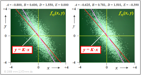
$\text{Example 3:}$ We always assume zero mean Gaussian random variables $u$ and $v$ Both have variance $σ^2 = 1$.

$(1)$ To generate a 2D random variable with the desired characteristics $σ_x =1$, $σ_y = 1.55$ and $ρ_{xy} = -0.8$ the parameter set is suitable, for example.

2D random variables generated by linear combination

$$A = -0.8, \; B = 0.6, \; D = 1.55, \; E = 0.$$

This set of parameters underlies the left graph.
The regression line $K(x)$ is shown in red.
It runs at an angle of about $-50^\circ$.
Drawn in purple is the ellipse major axis, which lies slightly above the regression line.

$(2)$ The parameter set for the right graph is:

$$A = -0.625,\; B = 0.781,\; D = 1.501,\; E = -0.390.$$

In a statistical sense, the same result is obtained even though the two point clouds differ in detail.
In particular, with respect to regression line and ellipse major axis, there is no difference with respect to the parameter set $(1)$.

Exercises for the chapter

Exercise 4.7: Weighted Sum and Difference

Exercise 4.7Z: Generation of a "2D-PDF"

Exercise 4.8: Diamond shaped "2D-PDF"

Exercise 4.8Z: AWGN Channel

Linear Combinations of Random Variables

Contents

Prerequisites and mean values

Resulting correlation coefficient

Generation of correlated random variables

Exercises for the chapter