Graphical Convolution

Open Applet in new Tab Deutsche Version Öffnen

Applet Description

This applet illustrates the convolution operation in the time domain

between an input pulse $x(t)$ ⇒ rectangle, triangle, Gaussian, exponential function
and the impulse response $h(t)$ of an LTI system with low–pass character ⇒ slit low–pass, first or second order low–pass, Gaussian low–pass.

For the output signal $y(t)$ corresponding to the block diagram in $\text{Example 1}$, then, as stated in the chapter "Graphical Convolution":

$$y( t ) = x(t) * h( t ) = \int_{ - \infty }^{ + \infty } \hspace{-0.15cm}{x( \tau )} \cdot h( {t - \tau } )\hspace{0.1cm}{\rm d}\tau .$$

For causal systems ⇒ $h(t) \equiv 0$ for $t < 0$ (examples: slit low–pass as well as first and second order low–pass) can be written for this also:

$$y( t ) = \int_{ - \infty }^{ t } \hspace{-0.15cm}{x( \tau )} \cdot h( {t - \tau } )\hspace{0.1cm}{\rm d}\tau .$$

Please note:

All quantities – also the time $t$ – are to be understood normalized (dimensionless).
The time functions $x(t)$, $h(t)$ and $y(t)$ cannot assume negative signal values in the program.
The absolute duration of a pulse $y(t)$ is the (continuous) time range for which $y(t) > 0$.
The equivalent duration of a pulse can be calculated by the rectangle of equal area.

Theoretical Background

Convolution in the time domain

The "convolution theorem" is one of the most important laws of the Fourier transform. We first consider the convolution theorem in the time domain and assume that the spectra of two time functions $x_1(t)$ and $x_2(t)$ are known:

$$X_1 ( f )\hspace{0.15cm}\bullet\!\!\!-\!\!\!-\!\!\!-\!\!\circ\hspace{0.15cm}x_1( t ),\quad X_2 ( f )\hspace{0.1cm}\bullet\!\!\!-\!\!\!-\!\!\!-\!\!\circ\hspace{0.1cm}x_2 ( t ).$$

Then for the time function of the product $X_1(f) \cdot X_2(f)$ holds:

$$X_1 ( f ) \cdot X_2 ( f )\hspace{0.15cm}\bullet\!\!\!-\!\!\!-\!\!\!-\!\!\circ\hspace{0.15cm}\int_{ - \infty }^{ + \infty } {x_1 ( \tau )} \cdot x_2 ( {t - \tau } )\hspace{0.1cm}{\rm d}\tau.$$

Here $\tau$ is a formal integration variable with the dimension of a time.

$\text{Definition:}$ The above connection of the time function $x_1(t)$ and $x_2(t)$ is called convolution and represents this functional connection with a star:

$$x_{\rm{1} } (t) * x_{\rm{2} } (t) = \int_{ - \infty }^{ + \infty } {x_1 ( \tau ) } \cdot x_2 ( {t - \tau } ) \hspace{0.1cm}{\rm d}\tau.$$

Thus, above Fourier correspondence can also be written as follows:

$$X_1 ( f ) \cdot X_2 ( f )\hspace{0.15cm}\bullet\!\!\!-\!\!\!-\!\!\!-\!\!\circ\hspace{0.15cm}{ {x} }_{\rm{1} } ( t ) * { {x} }_{\rm{2} } (t ).$$

$\text{Proof}$

Note: The convolution is commutative ⇒ The order of the operands is interchangeable: ${ {x}}_{\rm{1}} ( t ) * { {x}}_{\rm{2}} (t ) ={ {x}}_{\rm{2}} ( t ) * { {x}}_{\rm{1}} (t ) $.

For the calculation of signal and spectrum at the LTI output

$\text{Example 1:}$ Any linear time-invariant (LTI) system can be described both by the frequency response $H(f)$ and by the impulse response $h(t)$, the relationship between these two system quantities also being given by the Fourier transform.

If a signal $x(t)$ with the spectrum $X(f)$ is applied to the input, the following applies to the spectrum of the output signal:

$$Y(f) = X(f) \cdot H(f)\hspace{0.05cm}.$$

With the convolution theorem it is now possible to calculate the output signal also directly in the time domain:

$$y( t ) = x(t) * h( t ) = \int_{ - \infty }^{ + \infty } \hspace{-0.15cm}{x( \tau )} \cdot h( {t - \tau } )\hspace{0.1cm}{\rm d}\tau = \int_{ - \infty }^{ + \infty } \hspace{-0.15cm} {h( \tau )} \cdot x( {t - \tau } )\hspace{0.1cm}{\rm d}\tau = h(t) * x( t ).$$

From this equation, it is again clear that the convolution operation is commutative.

Convolution in the frequency domain

The duality between the time and frequency domains also allows us to make statements regarding the spectrum of a product signal:

$$x_1 ( t ) \cdot x_2 ( t )\circ\!\!-\!\!\!-\!\!\!-\!\!\bullet\,X_1 (f) * X_2 (f) = \int_{ - \infty }^{ + \infty } {X_1 ( \nu )} \cdot X_2 ( {f - \nu })\hspace{0.1cm}{\rm d}\nu.$$

This result can be proved similarly to the "convolution theorem in the time domain". However, the integration variable $\nu$ now has the dimension of a frequency.

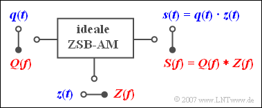
Convolution in the frequency domain

$\text{Example 2:}$ The "double-sideband amplitude modulation" (DSB-AM) without carrier is described by the sketched model.

In the time domain representation (blue), the modulated signal $s(t)$ is the product of the message signal $q(t)$ and the (normalized) carrier signal $z(t)$.
According to the convolution theorem, it follows for the frequency domain (red) that the output spectrum $S(f)$ is equal to the convolution product of $Q(f)$ and $Z(f)$.

Convolution of a function with a Dirac function

The convolution operation becomes very simple if one of the two operands is a "Dirac function". This is equally true for convolution in the time and frequency domain.

As an example, we consider the convolution of a function $x_1(t)$ with the function

$$x_2 ( t ) = \alpha \cdot \delta ( {t - T} ) \quad \circ\,\!\!\!-\!\!\!-\!\!\!-\!\!\bullet \quad X_2 ( f )= \alpha \cdot {\rm{e}}^{ - {\rm{j}}\hspace{0.03cm}2\hspace{0.03cm}{\rm{\pi }}\hspace{0.01cm}f\hspace{0.01cm}T}.$$

Then for the spectral function of the signal $y(t) = x_1(t) \ast x_2(t)$ holds:

$$Y( f ) = X_1 ( f ) \cdot X_2 ( f ) = X_1 ( f ) \cdot \alpha \cdot {\rm{e}}^{ - {\rm{j}}\hspace{0.03cm}2\hspace{0.03cm}{\rm{\pi }}\hspace{0.01cm}f\hspace{0.01cm}T} .$$

The complex exponential function leads to a shift by $T$ ⇒ "shifting theorem", the factor $\alpha$ to an attenuation $(\alpha < 1)$ or an amplification $(\alpha > 1)$. It follows that:

$$x_1 (t) * x_2 (t) = \alpha \cdot x_1 ( {t - T} ).$$

$\text{In words: }$ The convolution of an arbitrary function with a Dirac function at $t = T$ results in the function shifted to the right by $T$, whereby the weighting of the Dirac function by the factor $\alpha$ must still be taken into account.

$\text{Example 3:}$ A rectangular signal $x(t)$ is delayed by a running time $\tau = 3\,\text{ ms}$ and attenuated by a factor $\alpha = 0.5$ by an LTI system.

Convolution of a rectangle with a Dirac function

Shift and attenuation can be seen in the output signal $y(t)$ as well as in the impulse response $h(t)$.

Graphical Convolution

This applet assumes the following convolution operation:

Screen capture of the program "Graphical Convolution" (former version)

$$y(t) = x (t) * h (t) = \int_{ - \infty }^{ + \infty } {x ( \tau )} \cdot h ( {t - \tau } )\hspace{0.1cm}{\rm d}\tau.$$

The solution of the convolution integral is to be done graphically. It is assumed that $x(t)$ and $h(t)$ are continuous-time signals.

Then the following steps are required:

Change the time variables of the two functions:
$x(t) \to x(\tau)$, $h(t) \to h(\tau)$.
Mirror second function: $h(\tau) \to h(-\tau)$.
Shift mirrored function by $t$: $h(-\tau) \to h(t-\tau)$.
Multiplikation der beiden Funktionen $x(\tau)$ und $h(t-\tau)$.
Integration über das Produkt bezüglich $\tau$ in den Grenzen von $-\infty$ bis $+\infty$.

Da die Faltung kommutativ ist, kann anstelle von $h(\tau)$ auch $x(\tau)$ gespiegelt werden.

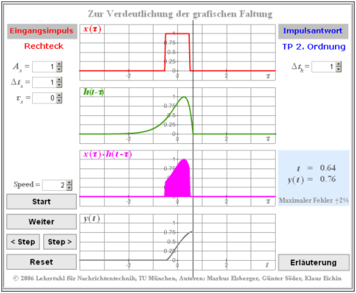
Nebenstehende Grafik zeigt einen Bildschirmabzug einer älteren Version des vorliegenden Applets.

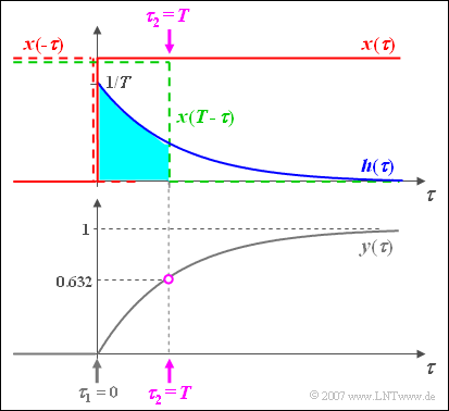
Beispiel einer Faltungsoperation:
Sprungfunktion gefaltet mit Exponentialfunktion

$\text{Beispiel 4:}$ Die Vorgehensweise bei der grafischen Faltung wird nun anhand eines ausführlichen Beispiels erklärt:

Am Eingang eines Filters liege eine Sprungfunktion $x(t) = \gamma(t)$ an.
Die Impulsantwort des RC-Tiefpasses sei $h( t ) = {1}/{T} \cdot {\rm{e} }^{ - t/T}.$

Die Grafik zeigt rot das Eingangssignal $x(\tau)$, blau die Impulsantwort $h(\tau)$ und grau das Ausgangssignal $y(\tau)$. Die Zeitachse ist bereits in $\tau$ umbenannt.

Das Ausgangssignal kann zum Beispiel nach folgender Gleichung berechnet werden:

$$y(t) = h(t) * x(t) = \int_{ - \infty }^{ + \infty } {h( \tau )} \cdot x( {t - \tau } )\hspace{0.1cm}{\rm d}\tau.$$

Noch einige Anmerkungen zur grafischen Faltung:

Der Ausgangswert bei $t = 0$ ergibt sich, indem man das Eingangssignal $x(\tau)$ spiegelt, dieses gespiegelte Signal $x(-\tau)$ mit der Impulsantwort $h(\tau)$ multipliziert und darüber integriert.
Da es hier kein Zeitintervall gibt, bei dem sowohl die blaue Kurve $h(\tau)$ und gleichzeitig auch die rot gestrichelte Spiegelung $x(-\tau)$ ungleich Null ist, folgt daraus $y(t=0)=0$.
Für jeden anderen Zeitpunkt $t$ muss das Eingangssignal verschoben werden ⇒ $x(t-\tau)$, beispielsweise entsprechend der grün gestrichelten Kurve für $t=T$.
Da in diesem Beispiel auch $x(t-\tau)$ nur die Werte $0$ oder $1$ annehmen kann, wird die Integration $($allgemein von $\tau_1$ bis $\tau_2)$ einfach und man erhält mit $\tau_1 = 0$ und $\tau_2 = t$ :

$$y( t) = \int_0^{\hspace{0.05cm} t} {h( \tau)}\hspace{0.1cm} {\rm d}\tau = \frac{1}{T}\cdot\int_0^{\hspace{0.05cm} t} {{\rm{e}}^{ - \tau /T } }\hspace{0.1cm} {\rm d}\tau = 1 - {{\rm{e}}^{ - t /T } }.$$

Die Skizze gilt für $t=T$ und führt zum Ausgangswert $y(t=T) = 1 – 1/\text{e} \approx 0.632$.

Exercises

First, select the number $(1,\ 2, \text{...} \ )$ of the task KORREKTUR: exercise to be processed. The number $0$ corresponds to a "Reset": Same setting as at program start.
A task KORREKTUR: An exercise description is displayed. The parameter values are adjusted. Solution after pressing "Show Solution".
Both the input signal $x(t)$ and the impulse response $h(t)$ of the filter are are normalized, dimensionless and energy-limited ("time-limited pulses").

(1) Select the following parameters: $\text{Gaussian pulse: }A_x = 1, \ \Delta t_x= 1, \ \tau_x = 1; \text{ Impulse response according to 2nd order low-pass: } \Delta t_h= 1$.
Interpret the displayed graphs. What is the maximum output value $y_{\rm max}$? At what time $t_{\rm max}$ does $y_{\rm max}$ occur?

After renaming: Input signal $x(\tau)$ ⇒ red curve, impulse response $h(\tau)$ ⇒ blue curve, after mirroring $h(-\tau)$ ⇒ green curve.
Shifting the green curve by $t$ to the right, we get $h(t-\tau)$. The output signal $y(t)$ is obtained by multiplication and integration with respect to $\tau$:

$$y (t) = \int_{ - \infty }^{ +\infty } {x ( \tau ) } \cdot h ( {t - \tau } ) \hspace{0.1cm}{\rm d}\tau = \int_{ - \infty }^{ t } {x ( \tau ) } \cdot h ( {t - \tau } ) \hspace{0.1cm}{\rm d}\tau .$$

The output pulse $y(t)$ is asymmetric in the present case; the maximum output value $y_{\rm max}\approx 0.67$ occurs at $t_{\rm max}\approx 1.5$.

(2) What changes if we increase the equivalent pulse duration of $h(t)$ to $\Delta t_h= 1.5$?

$y_{\rm max}\approx 0.53$ now occurs at $t_{\rm max}\approx 1.75$. Due to the less favorable (wider) impulse response, the input pulse is more deformed.
In a digital communication system, this would result in stronger "intersymbol interferences".

(3) Now select the symmetric $\text{rectangular pulse: }A_x = 1, \ \Delta t_x= 1, \ \tau_x = 0$ and the $\text{rectangular impulse response}$ of the low-pass filter: $\Delta t_h= 1$.
Interpret the convolution result. What is the maximum output value $y_{\rm max}$? At what times is $y(t)>0$? Does $h(t)$ describe a causal system?

The convolution of two rectangles with respective durations $1$ yields a triangle with absolute duration $2$ ⇒ equivalent pulse duration $\Delta t_y= 1$.
$y(t)$ is different from zero in the range from $-0.5$ to $+1.5$ . The pulse maximum $y_{\rm max} = 1$ is at $t_{\rm max} = +0.5$.
$h(t)$ describes a causal system, since $h(t) \equiv 0$ for $t < 0$. That means: The "effect" $y(t)$ does not come before the "cause" $x(t)$.

(4) What changes if we increase the equivalent pulse duration of $h(t)$ to $\Delta t_h= 2$ ?

The convolution of two rectangles of different widths results in a trapezoid, here between $-0.5$ and $+2.5$ ⇒ equivalent pulse duration $\Delta t_y= 2$.
The maximum $y_{\rm max} = 0.5$ occurs in the range $0.5 \le t \le 1.5$. Nothing changes with respect to causality.

(5) Now select the (unsymmetrical) $\text{rectangular pulse: }A_x = 1, \ \Delta t_x= 1, \ \tau_x = 0.5$ and the $\text{impulse response of a 1st order low-pass: }\Delta t_h= 1$.
Interpret the results. What is the value of $y_{\rm max}$? At what times is $y(t)>0$ ? Does $h(t)$ describe a causal system?

$h(t)$ has an exponentially decreasing curve for $t > 0$. It always applies: $y(t>0) > 0$, but the signal values can become very small.
$y_{\rm max} = 0.63$ occurs for $t_{\rm max} = +1$. For $ t < t_{\rm max}$ the progression is exponentially increasing, for $ t > t_{\rm max}$ exponentially decreasing.
The 1st order low-pass can be realized with a resistor and a capacitor. Any realizable system is causal per se.

(6) Select as in $(3)$ the $\text{rectangular impulse response}$ of the low-pass filter: $\Delta t_h= 1$. With which $x(t)$ results the same $y(t)$ as for $(5)$?

The signal $y(t)$ in $(5)$ resulted as a convolution between the rectangular input $x(t)$ and the exponential function $h(t)$.
Since the convolution operation is commutative, the same result is obtained with the exponential function $x(t)$ and the rectangular function $h(t)$.
Thus, the correct setting for the input signal $x(t)$ is the $\text{exponential pulse }$with $ A_x = 1, \ \Delta t_x= 1, \ \tau_x = 0$ .

(7) For the remainder of the exercises, we consider the Gaussian low-pass. The equivalent duration of the impulse response $h(t)$ should first be $\Delta t_h= 0.8$.
Analyze and interpret this "system" in terms of causality and the resulting distortions for the rectangular pulse.

The low-pass is not causal (and therefore non–realizable): For $t < 0$ does $h(t) \equiv 0$ not hold. KORREKTUR: $h(t) \equiv 0$ does not hold. Suitable model if infinite delay is ignored.
The larger $\Delta t_h$ is, the wider the output pulse and the stronger the degradation of a digital system due to intersymbol interference.
The frequency response $H(f)$ is the Fourier transform of $h(t)$. The larger $\Delta t_h$ is, the smaller $\Delta f_h = 1/\Delta t_h$ ⇒ The system is more narrowband.

(8) Now select $\text{Gaussian pulse: }A_x = 1, \ \Delta t_x= 1.5, \ \tau_x = 0$ and $\text{Gaussian low-pass: }\Delta t_h= 2$. What is the course of the output pulse $y(t)$?
What are the equivalent duration $\Delta t_y$ of the output pulse and the maximum output value $y_{\rm max}$? At what time $t_{\rm max}$ does $y_{\rm max}$ occur?

$y(t)$ is (exactly) Gaussian, too. Mnemonic: $\text{"Gaussian convolved with Gaussian gives always Gaussian"}$.
Equivalent duration: $\Delta t_y =\sqrt{\Delta t_x^2+ \Delta t_h^2} = 2.5$. Pulse maximum $($at $t=0)$: $y_{\rm max} = A_x \cdot \Delta t_x/\Delta t_y = 1 \cdot 1.5/2.5 = 0.6$.

(9) Now select $\text{Triangular pulse: }A_x = 1, \ \Delta t_x= 1.5, \ \tau_x = 0$ and $\text{Gaussian low–pass: }\Delta t_h= 2$. What is the course of the output pulse $y(t)$?
What is the equivalent duration $\Delta t_y$ of the output pulse and the maximum output value $y_{\rm max}$? At what time $t_{\rm max}$ does $y_{\rm max}$ occur?

$y(t)$ is nearly Gaussian, but not exactly. Mnemonic: $\text{"Gaussian convolved with non–Gaussian never gives exactly Gaussian"}$.
The characteristics of the output pulse $y(t)$ differ only slightly from $(8)$: $\Delta t_y \approx 2.551$, $y_{\rm max} \approx 0.588$.

Applet Manual

Screen shot (German version)

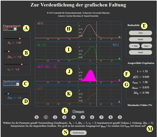
(A) Selection: Shape of the input pulse $x(t)$

(B) Parameter input for the input pulse $x(t)$

(C) Selection: Shape of the impulse response $h(t)$ of the low-pass system

(D) Parameter input for the impulse response $h(t)$

(E) Control panel (Start; Pause/Continue ; Step > ; Step < ; Reset)

(F) Output the initial value $y(t)$ at the continuous time $t$

(G) Maximum value $y_{\rm max} = y(t_{\rm max})$ and equivalent width $\Delta\hspace{0.03cm} t_y$

After renaming the abscissa: $t \ \to \ \tau$:

(H) Representation of $x(\tau)$ ⇒ red static curve.

(I) Representation of $h(\tau)$ ⇒ blue curve and $h(t-\tau)$ ⇒ green curve
$($this is shifted to the right with the motion parameter $t$ $)$

(J) Plot of $x(\tau) \cdot h(t - \tau)$ ⇒ purple curve, dynamic with $t$

(K) Successive representation of the output signal $y(t)$ ⇒ brown curve

(L) Area for exercise execution: Task KORREKTUR: Exercise selection.

(M) Exercise execution: Area for task KORREKTUR: exercise description

(N) Exercise execution: Area for the sample solution

About the Authors

This interactive calculation tool was designed and implemented at the Institute for Communications Engineering at the Technical University of Munich.

The first version was created in 2006 by Markus Elsberger as part of his bachelor thesis with “FlashMX – Actionscript” (Supervisor: Günter Söder).

Last revision and English version 2020/2021 by Carolin Mirschina in the context of a working student activity. Translation using DEEPL.com.

The conversion of this applet to HTML 5 was financially supported by Studienzuschüsse ("study grants") of the TUM Faculty EI. We thank. KORREKTUR: Many thanks.

Once again: Open Applet in new Tab

Open Applet in new Tab Deutsche Version Öffnen

Graphical Convolution

Contents

Applet Description

Theoretical Background

Convolution in the time domain

Convolution in the frequency domain

Convolution of a function with a Dirac function

Graphical Convolution

Exercises

Applet Manual

About the Authors

Once again: Open Applet in new Tab