Exercise 1.7: PDF of Rice Fading

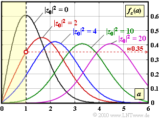
Rice fading for different values of $|z_0|^2$

As you can see in the diagram, we consider the same scenario as in Exercise 1.6:

Rice fading with variance of the Gaussian processes $\sigma^2 = 1$ and parameter $|z_0|$ for the direct path.
Regarding direct path, we are interested in the parameter values $|z_0|^2 = 0, \ 2, \ 4, \ 10, \ 20$ (see graph).
The PDF of the magnitude $a(t) = |z(t)|$ is

$$f_a(a) ={a}/{\sigma^2} \cdot {\rm e}^{ -{(a^2+ |z_0|^2) }/({2\sigma^2})}\cdot {\rm I}_0 \left [ {a \cdot |z_0|}/{\sigma^2} \right ]\hspace{0.05cm}.$$

For example, the modified zeroth order Bessel function returns the following values:

$${\rm I }_0 (2) = 2.28\hspace{0.05cm},\hspace{0.2cm}{\rm I }_0 (4) = 11.30\hspace{0.05cm},\hspace{0.2cm}{\rm I }_0 (3) = 67.23 \hspace{0.05cm}.$$

The power (noncentral second moment) of the multiplicative factor $|z(t)|$ is

$${\rm E}\left [ a^2 \right ] = {\rm E}\left [ |z(t)|^2 \right ] = 2 \cdot \sigma^2 + |z_0|^2 \hspace{0.05cm}.$$

With $z_0 = 0$, the Rice fading becomes Rayleigh fading, which is more critical. In this case, the probability that $a$ lies in the yellow-shaded area between $0$ and $1$ is

$$ {\rm Pr}(a \le 1) = 1 - {\rm e}^{-0.5/\sigma^2} \approx 0.4 \hspace{0.05cm}.$$

In this task the probability ${\rm Pr}(a ≤ 1)$ for $|z_0| ≠ 0$ is to be approximated. There are two ways to do this, namely:

the triangular approximation: ${\rm Pr}(a \le 1) = {1}/{2} \cdot f_a(a=1) \hspace{0.05cm}.$
the Gaussian approximation: If $|z_0| \gg \sigma$, then the Rice distribution can be approximated by a Gaussian distribution with mean $|z_0|$ and standard deviation $\sigma$ .

Notes:

This task belongs to chapter Non-frequency selective fading with direct component.
For the numerical solutions of the last subtasks, we recommend the interaction module Complementary Gaussian Error Functions.

Questions

$f_a(a = 1) \ = \ $

$f_a(a = 2) \ = \ $

$f_a(a = 3) \ = \ $

${\rm Pr}(a ≤ 1)\ = \ $

$\ \%$

${\rm Pr}(a ≤ 1) \ = \ $

$\ \%$

${\rm Pr}(a ≤ 1) \ = \ $

$\ \%$

${\rm Pr}(a ≤ 1) \ = \ $

$\ \%$

Solutions

Solution

(1) With $|z_0| = 2$ and $\sigma = 2$ the Rice PDF is $$f_a(a) = a \cdot {\rm exp} [ -\frac{a^2 + 4}{2}] \cdot {\rm I}_0 (2a)\hspace{0.05cm}.$$

This gives the desired values:

$$f_a(a = 1) \hspace{-0.1cm} \ = \ \hspace{-0.1cm} 1 \cdot {\rm e}^{-2.5} \cdot {\rm I}_0 (2) = 0.082 \cdot 2.28 \hspace{0.15cm} \underline{ = 0.187}\hspace{0.05cm},$$

$$f_a(a = 2) \hspace{-0.1cm} \ = \ \hspace{-0.1cm} 2 \cdot {\rm e}^{-4} \cdot {\rm I}_0 (4) = 2 \cdot 0.0183 \cdot 11.3 \hspace{0.15cm} \underline{ = 0.414}\hspace{0.05cm},$$

$$f_a(a = 3) \hspace{-0.1cm} \ = \ \hspace{-0.1cm} 3 \cdot {\rm e}^{-6.5} \cdot {\rm I}_0 (6) = 3 \cdot 0.0015 \cdot 67.23 \hspace{0.15cm} \underline{ = 0.303}\hspace{0.05cm}.$$

The results fit well with the blue curve on the graph.

(2) With the result of the subtask (1) ⇒ $f_a(a = 1) = 0.187$ the triangle approximation gives $${\rm Pr}(a \le 1) = {1}/{2} \cdot 0.187 \cdot 1\hspace{0.15cm} \underline{ \approx 9.4\,\%} \hspace{0.05cm}.$$

This result will be a bit too large, because the blue curve is below the connecting line from $(0, 0)$ to $(1, 0.187)$ ⇒ convex curve.

(3) For the red curve the WDF–value $f_a(a = 1) \approx 0.35$ can be read from the graph: $${\rm Pr}(a \le 1) = \frac{1}{2} \cdot 0.35 \hspace{0.15cm} \underline{ \approx 17.5\,\%} \hspace{0.05cm}.$$

The actual probability value will be slightly larger because the red curve is concave in the range between $0$ and $1$.

(4) The Gaussian approximation states that one can approximate the Rice distribution by a Gaussian distribution with mean $|z_0| = \sqrt{10} = 3.16$ and standard deviation $\sigma = 1$ if the quotient $|z_0|/\sigma$ is sufficiently large. Then we have $${\rm Pr}(a \le 1) \approx {\rm Pr}(g \le -2.16) = {\rm Q}(2.16) \hspace{0.15cm} \underline{ \approx 1.5\,\%} \hspace{0.05cm}.$$

Here, $g$ denotes a Gaussian distributed random variable with mean $0$ and standard deviation $\sigma = 1$.
The numerical value was determined with the specified interactive Applet.

Note: The Gaussian approximation is certainly associated with a certain error here:

From the graph you can see that the average value of the green curve is not $a = 3.16$ , but rather $3.31$.
Then the power of the Gaussian approximation $(3.31^2 + 1^2 = 12)$ is exactly the same as that of the Rice distribution:

$$|z_0|^2 + 2 \sigma^2= 10 + 2 =12\hspace{0.05cm}.$$

(5) Using the same calculation method, replace the Rice PDF with a Gaussian PDF with mean value $\sqrt{20} \approx $4.47 and standard deviation $\sigma = $1 and you get $${\rm Pr}(a \le 1) \approx {\rm Pr}(g \le -3.37) = {\rm Q}(3.37) { \approx 0.04\,\%} \hspace{0.05cm}.$$

If one assumes the equal power Gaussian distribution (see the note to the last subtask), the mean value is $m_g = \sqrt{21}\approx 4.58$, and the probability would then be

$${\rm Pr}(a \le 1) \approx {\rm Q}(3.58) \hspace{0.15cm} \underline{ \approx 0.02\,\%} \hspace{0.05cm}.$$