Moments of a Discrete Random Variable

Calculation as ensemble average or time average

The probabilities and the relative frequencies provide extensive information about a discrete random variable.

Reduced information is obtained by the so-called moments $m_k$, where $k$ represents a natural number.

$\text{Two alternative ways of calculation:}$

Under the condition "Ergodicity" implicitly assumed here, there are two different calculation possibilities for the $k$-th order moment:

the ensemble averaging or "expected value formation" ⇒ averaging over all possible values $\{ z_\mu\}$ with the index $\mu = 1 , \hspace{0.1cm}\text{ ...} \hspace{0.1cm} , M$:

$$m_k = {\rm E} \big[z^k \big] = \sum_{\mu = 1}^{M}p_\mu \cdot z_\mu^k \hspace{2cm} \rm with \hspace{0.1cm} {\rm E\big[\text{ ...} \big]\hspace{-0.1cm}:} \hspace{0.3cm} \rm expected\hspace{0.1cm}value ;$$

the time averaging over the random sequence $\langle z_ν\rangle$ with the index $ν = 1 , \hspace{0.1cm}\text{ ...} \hspace{0.1cm} , N$:

$$m_k=\overline{z_\nu^k}=\hspace{0.01cm}\lim_{N\to\infty}\frac{1}{N}\sum_{\nu=\rm 1}^{\it N}z_\nu^k\hspace{1.7cm}\rm with\hspace{0.1cm}horizontal\hspace{0.1cm}line\hspace{-0.1cm}:\hspace{0.1cm}time\hspace{0.1cm}average.$$

Note:

Both types of calculations lead to the same asymptotic result for sufficiently large values of $N$.
For finite $N$, a comparable error results as when the probability is approximated by the relative frequency.

First order moment – linear mean – DC component

$\text{Definition:}$ With $k = 1$ we obtain from the general equation the first order moment ⇒ the linear mean:

$$m_1 =\sum_{\mu=1}^{M}p_\mu\cdot z_\mu =\lim_{N\to\infty}\frac{1}{N}\sum_{\nu=1}^{N}z_\nu.$$

The left part of this equation describes the ensemble averaging (over all possible values),

while the right equation gives the determination as time average.

In the context of signals, this quantity is also referred to as the "direct current" $\rm (DC)$ component.

DC component $m_1$ of a binary signal

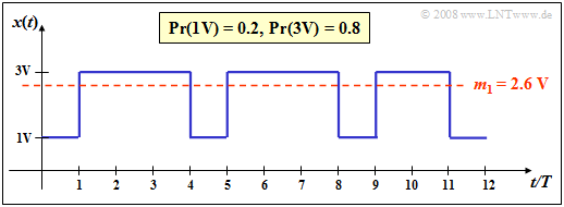
$\text{Example 1:}$ A binary signal $x(t)$ with the two possible values

$1\hspace{0.03cm}\rm V$ $($for the symbol $\rm L)$,
$3\hspace{0.03cm}\rm V$ $($for the symbol $\rm H)$

as well as the occurrence probabilities $p_{\rm L} = 0.2$ and $p_{\rm H} = 0.8$ has the linear mean ("DC component")

$$m_1 = 0.2 \cdot 1\,{\rm V}+ 0.8 \cdot 3\,{\rm V}= 2.6 \,{\rm V}. $$

This is drawn as a red line in the graph.

If we determine this parameter by time averaging over the displayed $N = 12$ signal values, we obtain a slightly smaller value:

$$m_1\hspace{0.01cm}' = 4/12 \cdot 1\,{\rm V}+ 8/12 \cdot 3\,{\rm V}= 2.33 \,{\rm V}. $$

Here, the probabilities $p_{\rm L} = 0.2$ and $p_{\rm H} = 0.8$ were replaced by the corresponding frequencies $h_{\rm L} = 4/12$ and $h_{\rm H} = 8/12$ respectively.
In this example the relative error due to insufficient sequence length $N$ is greater than $10\%$.

$\text{Note about our (admittedly somewhat unusual) nomenclature:}$

We denote binary symbols here as in circuit theory with $\rm L$ ("Low") and $\rm H$ ("High") to avoid confusion.

In coding theory, it is useful to map $\{ \text{L, H}\}$ to $\{0, 1\}$ to take advantage of the possibilities of modulo algebra.
In contrast, to describe modulation with bipolar (antipodal) signals, one better chooses the mapping $\{ \text{L, H}\}$ ⇔ $ \{-1, +1\}$.

Second order moment – power – variance – standard deviation

$\text{Definitions:}$

Analogous to the linear mean, $k = 2$ obtains the second order moment ("mean square"):

$$m_2 =\sum_{\mu=\rm 1}^{\it M}p_\mu\cdot z_\mu^2 =\lim_{N\to\infty}\frac{\rm 1}{\it N}\sum_{\nu=\rm 1}^{\it N}z_\nu^2.$$

Together with the DC component $m_1$ the variance $σ^2$ can be determined from this as a further parameter ("Steiner's theorem"):

$$\sigma^2=m_2-m_1^2.$$

The standard deviation $σ$ is the square root of the variance:

$$\sigma=\sqrt{m_2-m_1^2}.$$

$\text{Notes on units:}$

For a random signal $x(t)$ ⇒ $m_2$ gives the total power (DC power plus AC power) related to the resistance $1 \hspace{0.03cm} Ω$.
If $x(t)$ describes a voltage, accordingly $m_2$ has the unit ${\rm V}^2$ and the rms value ( "root mean square") $x_{\rm eff}=\sqrt{m_2}$ has the unit ${\rm V}$. The total power for any reference resistance $R$ is calculated to $P=m_2/R$ and accordingly has the unit $\rm V^2/(V/A) = W$.
If $x(t)$ describes a current waveform, then $m_2$ has the unit ${\rm A}^2$ and the rms value $x_{\rm eff}=\sqrt{m_2}$ has the unit ${\rm A}$. The total power for any reference resistance $R$ is calculated to $P=m_2\cdot R$ and accordingly has the unit $\rm A^2 \cdot(V/A) = W$.
Only in the special case $m_1=0$ ⇒ the variance is $σ^2=m_2$. Then the standard deviation $σ$ coincides also with the rms value $x_{\rm eff}$ .

The following (German language) learning video illustrates the defined quantities using the example of a digital signal:
Momentenberechnung bei diskreten Zufallsgrößen ⇒ "Moment Calculation for Discrete Random Variables".

"Standard deviation" of a binary signal

$\text{Example 2:}$ For a binary signal $x(t)$ with the amplitude values.

$1\hspace{0.03cm}\rm V$ $($for the symbol $\rm L)$,
$3\hspace{0.03cm}\rm V$ $($for the symbol $\rm H)$

and the probabilities of occurrence $p_{\rm L} = 0.2$ resp. $p_{\rm H} = 0.8$ results for the second moment:

$$m_2 = 0.2 \cdot (1\,{\rm V})^2+ 0.8 \cdot (3\,{\rm V})^2 = 7.4 \hspace{0.1cm}{\rm V}^2,$$

The rms value $x_{\rm eff}=\sqrt{m_2}=2.72\,{\rm V}$ is independent of the reference resistance $R$ unlike the total power. For the latter, with $R=1 \hspace{0.1cm} Ω$ the value $P=7.4 \hspace{0.1cm}{\rm W}$, with $R=50 \hspace{0.1cm} Ω$ on the other hand, only $P=0.148 \hspace{0.1cm}{\rm W}$.

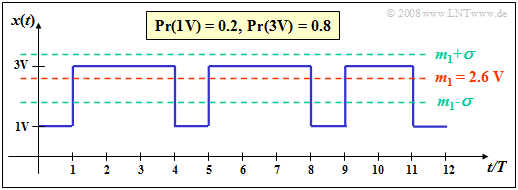
With the DC component $m_1 = 2.6 \hspace{0.05cm}\rm V$ $($see $\text{Example 1})$ it follows for

the variance $ σ^2 = 7.4 \hspace{0.05cm}{\rm V}^2 - \big [2.6 \hspace{0.05cm}\rm V\big ]^2 = 0.64\hspace{0.05cm} {\rm V}^2$,
the standard deviation $σ = 0.8 \hspace{0.05cm} \rm V$.

The same variance $ σ^2 = 0.64\hspace{0.05cm} {\rm V}^2$ and the same standard deviation $σ = 0.8 \hspace{0.05cm} \rm V$ result for the amplitudes $0\hspace{0.05cm}\rm V$ $($for the symbol $\rm L)$ and $2\hspace{0.05cm}\rm V$ $($for the symbol $\rm H)$, provided the occurrence probabilities $p_{\rm L} = 0.2$ and $p_{\rm H} = 0.8$ remain the same. Only the DC component and the total power change:

$$m_1 = 1.6 \hspace{0.05cm}{\rm V}, $$

$$P = {m_1}^2 +\sigma^2 = 3.2 \hspace{0.05cm}{\rm V}^2.$$

Exercises for the chapter

Exercise 2.2: Multi-Level Signals

Exercise 2.2Z: Discrete Random Variables

Moments of a Discrete Random Variable

Contents

Calculation as ensemble average or time average

First order moment – linear mean – DC component

Second order moment – power – variance – standard deviation

Exercises for the chapter