Exercise 4.3: Natural and Discrete Sampling

For natural and discrete sampling

Ideal sampling can be described in time domain by multiplying the analog source signal $q(t)$ by a Dirac comb $p_δ(t)$ :

$$ q_{\rm A}(t) = p_{\delta}(t) \cdot q(t) \hspace{0.05cm}.$$

Dirac impulses – infinitely narrow and infinitely high – and accordingly also the "Dirac comb" $p_δ(t)$ cannot be realized in practice, however.

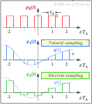
Here we must assume instead the "rectangular pulse comb" $p_{\rm R}(t)$ where the following relation holds:

$$ p_{\rm R}(t) = \left [ \frac{1}{T_{\rm A}} \cdot p_{\rm \delta}(t) \right ]\star g_{\rm R}(t)\hspace{0.4cm}\text{with}\hspace{0.4cm} g_{\rm R}(t) = \left\{ \begin{array}{l} 1 \\ 1/2 \\ 0 \\ \end{array} \right.\quad \begin{array}{*{5}c}{\rm{f\ddot{u}r}} \\{\rm{f\ddot{u}r}} \\{\rm{f\ddot{u}r}} \\ \end{array}\begin{array}{*{10}c} {\hspace{0.04cm}\left|\hspace{0.06cm} t \hspace{0.05cm} \right|} < T_{\rm R}/2\hspace{0.05cm}, \\ {\hspace{0.04cm}\left|\hspace{0.06cm} t \hspace{0.05cm} \right|} = T_{\rm R}/2\hspace{0.05cm}, \\ {\hspace{0.005cm}\left|\hspace{0.06cm} t \hspace{0.05cm} \right|} > T_{\rm R}/2\hspace{0.05cm}. \\ \end{array}$$

The duration $T_{\rm R}$ of a rectangular pulse $g_{\rm R}(t)$ should be (significantly) smaller than the distance $T_{\rm A}$ of two samples.

In the diagram this ratio is chosen with $T_{\rm R}/T_{\rm A} = 0.5$ very large to make the difference between "natural sampling" and "discrete sampling" especially clear:

In natural sampling, the sampled signal $q_{\rm A}(t)$ is equal to the product of the rectangular pulse comb $p_{\rm R}(t)$ and the analog source signal $q(t)$:

$$q_{\rm A}(t) = p_{\rm R}(t) \cdot q(t) = \left [ \frac{1}{T_{\rm A}} \cdot p_{\rm \delta}(t) \star g_{\rm R}(t)\right ]\cdot q(t)\hspace{0.05cm}.$$

In contrast, the corresponding equation for discrete sampling is:

$$ q_{\rm A}(t) = \left [ \frac{1}{T_{\rm A}} \cdot p_{\rm \delta}(t) \cdot q(t)\right ]\star g_{\rm R}(t)\hspace{0.05cm}.$$

In the graph, these signals are sketched in blue (natural sampling) and green (discrete sampling) respectively.

For signal reconstruction, a rectangular low-pass filter $H(f)$ with cutoff frequency $f_{\rm G} = f_{\rm A}/2$ and gain $T_{\rm A}/T_{\rm R}$ is used in the passband:

$$H(f) = \left\{ \begin{array}{l} T_{\rm A}/T_{\rm R} \\ 0 \\ \end{array} \right.\quad \begin{array}{*{5}c}{\rm{f\ddot{u}r}} \\{\rm{f\ddot{u}r}} \\ \end{array}\begin{array}{*{10}c} {\hspace{0.04cm}\left| \hspace{0.005cm} f\hspace{0.05cm} \right| < f_{\rm A}/2}\hspace{0.05cm}, \\ {\hspace{0.04cm}\left| \hspace{0.005cm} f\hspace{0.05cm} \right| > f_{\rm A}/2}\hspace{0.05cm}. \\ \end{array}$$

Hints:

The exercise belongs to the chapter "Pulse Code Modulation".
Reference is made in particular to the page "Natural and discrete sampling".
The sampled source signal is denoted by $q_{\rm A}(t)$ and its spectral function by $Q_{\rm A}(f)$.
Sampling is always performed at $ν \cdot T_{\rm A}$.

Questions

Solution

(1) The spectrum of the square pulse $g_{\rm R}(t)$ with amplitude $1$ and duration $T_{\rm R}$ is:

$$ G_{\rm R}(f) = T_{\rm R} \cdot {\rm si}(\pi f T_{\rm R}) \hspace{0.3cm} {\rm with}\hspace{0.3cm} {\rm si}(x) = \sin(x)/x \hspace{0.3cm} \rightarrow \hspace{0.3cm} \frac{G_{\rm R}(f)}{T_{\rm A}} = \frac{T_{\rm R}}{T_{\rm A}} \cdot {\rm si}(\pi f T_{\rm R})$$

$$ \rightarrow \hspace{0.3cm} \frac{G_{\rm R}(f = 0)}{T_{\rm A}} =\frac{T_{\rm R}}{T_{\rm A}}\hspace{0.15cm}\underline { = 0.5} \hspace{0.05cm}.$$

(2) The correct solution is the second suggested solution:

From the given equation in the time domain, the convolution theorem gives:

$$q_{\rm A}(t) = \left [ \frac{1}{T_{\rm A}} \cdot p_{\rm \delta}(t) \star g_{\rm R}(t)\right ]\cdot q(t) \hspace{0.3cm} \Rightarrow \hspace{0.3cm}Q_{\rm A}(f) = \left [ \frac{1}{T_{\rm A}}\cdot P_{\rm \delta}(f) \cdot G_{\rm R}(f) \right ] \star Q(f) = \left [ P_{\rm \delta}(f) \cdot \frac{G_{\rm R}(f)}{{T_{\rm A}}} \right ] \star Q(f) \hspace{0.05cm}.$$

The first proposed solution is valid only for ideal sampling (with a Dirac comb) and the last one for discrete sampling.

(3) The answer is YES:

Starting from the result of the subtask (2) using the spectral function of the Dirac comb, we obtain.

$$Q_{\rm A}(f) = \left [ P_{\rm \delta}(f) \cdot \frac{G_{\rm R}(f)}{{T_{\rm A}}} \right ] \star Q(f)= \left [ \frac{G_{\rm R}(f)}{{T_{\rm A}}} \cdot \sum_{\mu = -\infty}^{+\infty} \delta(f - \mu \cdot f_{\rm A})\right ] \star Q(f) \hspace{0.05cm}.$$

When the sampling theorem is satisfied and the low-pass filter is correct, of the infinite convolution products, only the convolution product with $μ = 0$ lie in the passband.
Taking into account the gain factor $T_{\rm A}/T_{\rm R}$ we thus obtain for the spectrum at the filter output:

$$V(f) = \frac{T_{\rm A}}{T_{\rm R}} \cdot \left [ \frac{G_{\rm R}(f = 0)}{{T_{\rm A}} \cdot \delta(f )\right ] \star Q(f)= Q(f) \hspace{0.05cm}.$$

(4) The last suggested solution is correct.

Shifting the factor $1/T_{\rm A}$ to the rectangular pulse, we obtain with discrete sampling using the convolution theorem:

$$ q_{\rm A}(t) = \big [ p_{\rm \delta}(t)\cdot q(t) \big ] \star \frac{g_{\rm R}(t)}{T_{\rm A}}\hspace{0.3cm} \Rightarrow \hspace{0.3cm}Q_{\rm A}(f)= \big [ P_{\rm \delta}(f)\star Q(f) \big ] \cdot \frac{G_{\rm R}(f)}{T_{\rm A}}\hspace{0.05cm}.$$

(5) The answer is NO:

The weighting function $G_{\rm R}(f)$ now involves the inner kernel $(μ = 0)$ of the convolution product.
All other terms $(μ ≠ 0)$ are eliminated by the low-pass filter. One obtains here in the relevant range $|f| < f_{\rm A}/2$:

$$V(f) = \frac{T_{\rm A}}{T_{\rm R}} \cdot \frac{G_{\rm R}(f )}{{T_{\rm A}}} \cdot Q(f) = 2 \cdot 0.5 \cdot {\rm si}(\pi f T_{\rm R})\cdot Q(f) \hspace{0.3cm}\Rightarrow \hspace{0.3cm}V(f) = Q(f) \cdot {\rm si}(\pi f T_{\rm R})\hspace{0.05cm}.$$

If no additional equalization is provided here, the higher frequencies are attenuated according to the $\rm si$ function.
The highest signal frequency $(f = f_{\rm A}/2)$ is attenuated the most here:

$$V(f = \frac{f_{\rm A}}{2}) = Q( \frac{f_{\rm A}}{2}) \cdot {\rm si}(\pi \cdot \frac{T_{\rm R}}{2 \cdot T_{\rm A}})= Q( \frac{f_{\rm A}}{2}) \cdot {\rm si}(\pi \cdot \frac{\sin(\pi/4)}{\pi/4})\approx 0.9 \cdot Q( \frac{f_{\rm A}}{2}) \hspace{0.05cm}.$$

	It holds $Q_{\rm A}(f) = P_{\rm δ}(f) ∗ Q(f)$.
	It holds $Q_{\rm A}(f) = \big[{\rm δ}(f) \cdot (G_{\rm R}(f)/T_{\rm A})\big] ∗ Q(f)$.
	It holds $Q_{\rm A}(f) = \big[P_{\rm δ}(f) ∗ Q(f)\big] \cdot (G_{\rm R}(f)/T_{\rm A})$.

	Yes.
	No.

	Yes.
	No.