Exercise 3.2Z: Optimum Cutoff Frequency for Gaussian Low-pass

Eye diagrams –
without and with noise

As in Exercise 3.2, a binary bipolar redundancy-free binary system with Gaussian receiver filter $H_{\rm G}(f)$ is considered. Its cutoff frequency $f_{\rm G}$ is to be determined such that the worst-case S/N ratio

$$\rho_{\rm U} = \frac{\big[\ddot{o}(T_{\rm D})/2 \big]^2}{ \sigma_d^2}\hspace{0.3cm}\Rightarrow \hspace{0.3cm} p_{\rm U} = {\rm Q} \left( \sqrt{\rho_{\rm U}} \right)$$

becomes maximum and thus the worst-case error probability $p_{\rm U}$ becomes minimum. The thus optimized cutoff frequency $f_{\rm G, \ opt}$ usually also leads to the minimum mean symbol error probability $p_{\rm S, \ min}$.

In the above equation, the following system quantities are used:

$\sigma_d^2$ is the detection noise power. For Gaussian receiver filters holds:

$$\sigma_d^2 = \frac{N_0}{2} \cdot \int_{-\infty}^{+\infty} |H_{\rm G}(f)|^2 \,{\rm d} f = \frac{N_0 \cdot f_{\rm G}}{\sqrt{2}}\hspace{0.05cm}.$$

$\ddot{o}(T_{\rm D})$ indicates the eye opening. The detection time is always assumed to be $T_{\rm D} = 0$.
For a Gaussian receiver filter, the vertical eye opening $\ddot{o}(T_{\rm D})$ can be expressed solely by the amplitude $s_0$ of the basic transmission pulse (upper boundary line in the eye diagram without noise) and the maximum value $g_0$ of the basic transmitter pulse.
The pulse amplitude $g_0$ is to be calculated as follows:

$$g_0 = g_d(t = 0) = s_0 \cdot \big [1- 2 \cdot {\rm Q} \left( \sqrt{2\pi} \cdot f_{\rm G} \cdot T \right)\big]\hspace{0.05cm}.$$

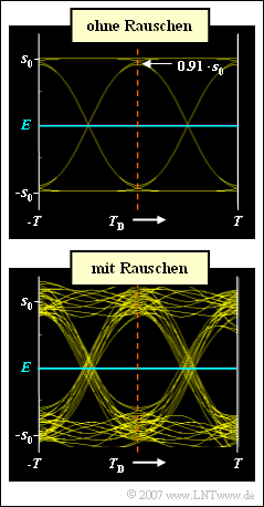
The graph shows the eye diagrams of the sought configuration with optimal cutoff frequency.

In the upper diagram, the noise interferences are not considered.
The lower diagram, on the other hand, is valid with AWGN noise for $10 \cdot {\rm lg} \ E_{\rm B}/N_0 = 10 \ \rm dB$.

Notes:

The exercise belongs to the chapter "Error Probability with Intersymbol Interference".
Use the interaction module "Complementary Gaussian Error Functions" for the numerical evaluation of the Q-function.

Questions

	The eye opening is calculated without noise.
	With Gaussian receiver filter, $\ddot{o}(T_{\rm D})/2 = s_0 \ – \ g_0$ is true.
	With Gaussian pulse shaper, $\ddot{o}(T_{\rm D})/2 = 2 \cdot g_0 \ – \ s_0$ is true.

$f_{\rm G, \ min} \cdot T \ = \ $

$f_{\rm G} \cdot T = 0.6\text{:} \hspace{0.4cm} 10 \cdot \rm lg \ \rho_{\rm U} \ = \ $

$\ \rm dB$

$f_{\rm G} \cdot T = 0.8\text{:} \hspace{0.4cm} 10 \cdot \rm lg \ \rho_{\rm U}\ = \ $

$\ \rm dB$

$f_{\rm G} \cdot T = 1.0\text{:} \hspace{0.4cm} 10 \cdot \rm lg \ \rho_{\rm U} \ = \ $

$\ \rm dB$

	Optimization with respect to $p_{\rm U}$ $($or $\rho_{\rm U})$ yields $f_{\rm G, \ opt} \cdot T \approx 0.8$.
	This optimization result is independent of $E_{\rm B}/N_0$.
	Optimization with respect to $p_{\rm S}$ leads to exactly the same result.

$\ddot{o}(T_{\rm D})/s_0 \ = \ $

$\sigma_d/s_0 \ = \ $

$10 \cdot \rm lg \ \rho_{\rm U} \ = \ $

$\ \rm dB$

$p_{\rm U}\ = \ $

$\ \cdot 10^{\rm -5}$

Solution

(1) The first and third solutions are correct:

When calculating the vertical eye opening, the noise component must not be taken into account. This is captured by the noise rms value $\sigma_d$.
If the eye opening were taken from the lower eye diagram, the noise component would be captured twice.
The upper boundary of the inner eye line results for the symbol sequence " $\text{ ...} \, \ -\hspace{-0.1cm}1 \ -\hspace{-0.1cm}1, +1, -\hspace{-0.1cm}1, \ -\hspace{-0.1cm}1, \text{ ...} $ " .
The long "$-1$" sequence would lead to the value $-s_0$.
In contrast, the "worst–case" sequence leads to the eye line $-s_0 + 2 \cdot g_d(t)$.
Thus, at detection time $T_{\rm D} = 0$, with decision threshold $E = 0$:

$${\ddot{o}(T_{\rm D})}/{ 2}= 2 \cdot g_0 - s_0 \hspace{0.05cm}.$$

(2) For the half vertical eye opening holds:

$${\ddot{o}(T_{\rm D})}/{ 2} \ = \ 2 \cdot g_0 - s_0 = 2 \cdot s_0 \cdot\left [ 1- 2 \cdot {\rm Q} \left( \sqrt{2\pi} \cdot f_{\rm G} \cdot T \right)\right] - s_0 = s_0 \cdot\left [ 1- 4 \cdot {\rm Q} \left( \sqrt{2\pi} \cdot f_{\rm G} \cdot T \right)\right] \hspace{0.05cm}.$$

A closed eye results according to the given interaction module for

$${\rm Q} \left( \sqrt{2\pi} \cdot f_{\rm G} \cdot T \right) \ge 0.25 \hspace{0.3cm}\Rightarrow \hspace{0.3cm} \sqrt{2\pi} \cdot f_{\rm G} \cdot T< 0.675\hspace{0.3cm}\Rightarrow \hspace{0.3cm} f_{\rm G, min} \cdot T \approx \frac{0.675}{2.5}\hspace{0.15cm}\underline { \approx 0.27} \hspace{0.05cm}.$$

(3) Using the equations on the information section and the previous calculations, we obtain

$\rho_{\rm U}$ as a function of (normalized) cutoff frequency

$$\rho_{\rm U} = \frac{[\ddot{o}(T_{\rm D})/2]^2}{ \sigma_d^2} = \frac{s_0^2 \cdot\left [ 1- 4 \cdot {\rm Q} \left( \sqrt{2\pi} \cdot f_{\rm G} \cdot T \right)\right]^2}{ N_0 \cdot f_{\rm G} / \sqrt{2}}$$

With the specification $E_{\rm B}/N_0 = 10 \ \rm dB $, the following determining equation is obtained:

$$10 \cdot {\rm lg}\hspace{0.1cm} {E_{\rm B}}/{ N_0} = 10 \, {\rm dB}\hspace{0.3cm}\Rightarrow \hspace{0.3cm} {E_{\rm B}}/{ N_0} = {s_0^2 \cdot T}/{ N_0} = 10$$

$$\Rightarrow \hspace{0.3cm} \rho_{\rm U} = 10 \cdot \sqrt{2} \cdot \frac{ \left [ 1- 4 \cdot {\rm Q} \left( \sqrt{2\pi} \cdot f_{\rm G} \cdot T \right)\right]^2}{ f_{\rm G} \cdot T}\hspace{0.05cm}.$$

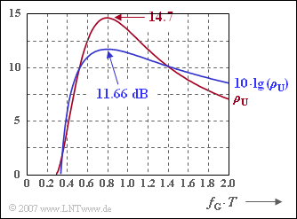
The figure shows this function plot as a function of the (normalized) cutoff frequency. For the given cutoff frequencies holds:

$f_{\rm G} \cdot T = 0.6\text{:} \hspace{0.4cm} \rho_{\rm U} \approx 12.7 \Rightarrow 10 \cdot \rm lg \ \rho_{\rm U} \ \underline {\approx \ 11.04 \ \rm dB},$
$f_{\rm G} \cdot T = 0.8\text{:} \hspace{0.4cm} \rho_{\rm U} \approx 14.7 \Rightarrow 10 \cdot \rm lg \ \rho_{\rm U} \ \underline {\approx \ 11.66 \ \rm dB},$
$f_{\rm G} \cdot T = 1.0\text{:} \hspace{0.4cm} \rho_{\rm U} \approx 13.5 \Rightarrow 10 \cdot \rm lg \ \rho_{\rm U} \ \underline {\approx \ 11.30 \ \rm dB}.$

From the above graph, one can also see the minimum cutoff frequency ⇒ subtask (2).

(4) The first two solutions are correct:

The validity of the first statement is evident from the above graph.
Since in the above equation for $\rho_{\rm U}$ the ratio $E_{\rm B}/N_0$ occurs only as a factor, the optimization (setting the derivative to zero) always leads to the same result independent of $E_{\rm B}/N_0$.
The optimal cutoff frequency with respect to $p_{\rm U}$ is approximately optimal with respect to $p_{\rm S}$ as well, but not exactly.
For very large values of $E_{\rm B}/N_0$ (small noise), this approximation is very correct and $p_{\rm S} \ \approx \ p_{\rm U}/4$ holds.
In contrast, for large noise, for example $10 \cdot {\rm lg} \ E_{\rm B}/N_0 = 0 \ \rm dB$, a smaller optimal cutoff frequency results when the optimization is based on $p_{\rm S}$:

$f_{\rm G} \cdot T = 0.8\text{:} \hspace{0.4cm} p_{\rm U} = 0.113, p_{\rm S} = 0.102,$

$f_{\rm G} \cdot T = 0.6\text{:} \hspace{0.4cm} p_{\rm U} = 0.129, p_{\rm S} = 0.094.$

However, the error probabilities are then so large that these results are not practically relevant.

(5) With the result of subtask (2) ⇒ $E_{\rm B}/N_0 = 10$ and $f_{\rm G} \cdot T = 0.8$ holds:

$${\ddot{o}(T_{\rm D})}/{ s_0} = 2 \cdot \left [ 1- 4 \cdot {\rm Q} \left( \sqrt{2\pi} \cdot 0.8 \right)\right] = 2 \cdot \left [ 1- 4 \cdot 0.022\right]\hspace{0.15cm}\underline { = 1.824} \hspace{0.05cm},$$

$${\sigma_d^2}/{ s_0^2} = \frac{N_0 \cdot f_{\rm G} }{\sqrt{2}\cdot s_0^2}= \frac{N_0 }{s_0^2 \cdot T} \cdot \frac{f_{\rm G} \cdot T}{\sqrt{2}} = 0.1 \cdot \frac{0.8}{\sqrt{2}} \approx 0.0566 \hspace{0.3cm}\Rightarrow \hspace{0.3cm}{\sigma_d}/{ s_0}\hspace{0.15cm}\underline { \approx 0.238} \hspace{0.05cm},$$

$$\rho_{\rm U} = \frac{[\ddot{o}(T_{\rm D})]^2}{ 4 \cdot \sigma_d^2} = \frac{1.824^2}{ 4 \cdot 0.0566}\approx 14.7 \hspace{0.3cm}\Rightarrow \hspace{0.3cm} 10 \cdot {\rm lg}\hspace{0.1cm} \rho_{\rm U}\hspace{0.15cm}\underline {\approx 11.66\, {\rm dB}} \hspace{0.05cm}.$$

$$p_{\rm U} = {\rm Q} \left( \sqrt{\rho_{\rm U}} \right) = {\rm Q} \left( \sqrt{14.7} \right) \hspace{0.15cm}\underline { \approx 6.4 \cdot 10^{-5}}\hspace{0.05cm}.$$