Carrier Frequency Systems with Non-Coherent Demodulation

Rayleigh and Rice Distribution

The estimation of the phase angle from the incoming signal, which is required for coherent demodulation, is not possible or only possible to a limited extent in many applications. For example, the movement of a mobile subscriber at high speed leads to very rapid temporal changes in the phase angle $\phi$, which makes its sufficiently accurate determination difficult or even impossible.

This fact leads to the non-coherent demodulation processes with the advantage of reduced complexity, but with increased error probability. In the derivation of the equations one encounters two probability density functions, which are given here in advance:

The Rayleigh distribution is obtained for the power density function $\rm (PDF)$ of the random variable $y$ with realization $\eta$, which is obtained from the two Gaussian distributed and statistically independent components $u$ and $v$ $($both with the same standard deviation $\sigma_n)$ as follows:

\[y = \sqrt{u^2 + v^2} \hspace{0.3cm} \Rightarrow \hspace{0.3cm} p_y (\eta) ={\eta}/{\sigma_n^2} \cdot {\rm exp } \left [ - {\eta^2}/{ (2\sigma_n^2)}\right ] \hspace{0.05cm}.\]

The Rice distribution is obtained under the same boundary conditions for the case where a constant $C$ is added to one of the components $($either to $u$ or $v)$:

\[y = \sqrt{(u+C)^2 + v^2} \hspace{0.3cm} \Rightarrow \hspace{0.3cm} p_y (\eta) = {\eta}/{\sigma_n^2} \cdot {\rm exp } \left [ - ({\eta^2 + C^2})/(2 \sigma_n^2) \right ] \cdot {\rm I }_0 \left [{\eta \cdot C}/{ \sigma_n^2}\right ] \hspace{0.05cm}.\]

The Rice distribution uses the "modified zero-order Bessel function", whose definition and series expansion are as follows:

\[{\rm I }_0 (x) = \frac{1}{ 2\pi} \cdot \int_{0}^{2\pi} {\rm e }^{-x \hspace{0.03cm}\cdot \hspace{0.03cm}\cos(\alpha)} \,{\rm d} \alpha \hspace{0.2cm} \approx \hspace{0.2cm} \sum_{k = 0}^{\infty} \frac{(x/2)^{2k}}{k! \cdot \Gamma (k+1)} \hspace{0.05cm}.\]

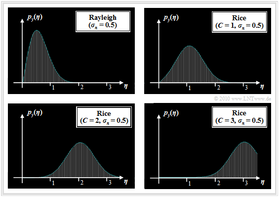
The graph shows the probability density functions of Rayleigh and Rice distributions. To this representation it is to be noted:

Rayleigh resp. Rice PDF for $σ_n = 0.5$

The Rice distribution is determined by the two parameters $C$ and $\sigma_n$. With $C = 0$, the Rice PDF is identical to the Rayleigh PDF.

The Rayleigh PDF with larger $\sigma_n$ is of the same shape as shown for $\sigma_n = 0.5$, but wider and lower in the ratio of standard deviation.

$\sigma_n$ indicates the standard deviation of the two Gaussian distributed random variables $u$ and $v$ and not the standard deviation of the Rayleigh distributed random variable $y$. Rather, the following applies to the latter:

\[\sigma_y = \sigma_n \cdot \sqrt{2 - {\pi}/{2 }} \hspace{0.2cm} \approx \hspace{0.2cm} 0.655 \cdot \sigma_n \hspace{0.05cm}.\]

The Rayleigh PDF is extremely asymmetric, recognizable by the large value for the "third order central moment" ⇒ "Charlier's skewness":

$$\mu_3/\sigma_y \approx 0.27.$$

The Rice PDF is more symmetrical the larger the quotient $C/\sigma_n$. For $C/\sigma_n \ge 4$: $\mu_3 \approx 0$ ⇒ symmetrical PDF.

The larger $C/\sigma_n$ is, the more the Rice PDF $($with $C$, $\sigma_n)$ approaches a "Gaussian PDF" with mean $C$ and standard deviation $\sigma_n$:

$$p_y (\eta) \approx \frac{1}{\sqrt{2\pi} \cdot \sigma_n} \cdot {\rm exp } \left [ - \frac{(\eta - C)^2}{2 \sigma_n^2}\right ]$$

$$ \Rightarrow \hspace{0.3cm} m_y = C\hspace{0.05cm},\hspace{0.2cm}\sigma_y = \sigma_n \hspace{0.05cm}.$$

Non-coherent demodulation of "on–off keying" (OOK)

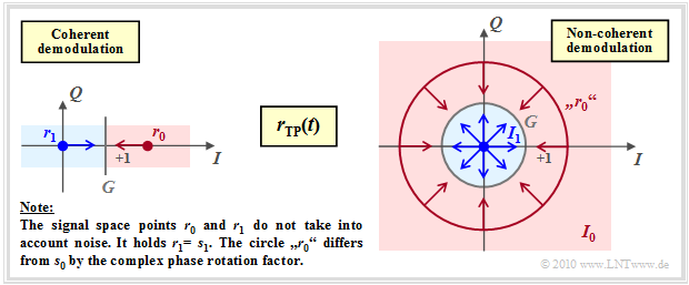
We consider "on–off keying" $(\rm OOK$ or $\rm 2–ASK)$ in the equivalent low-pass range.

Coherent and non-coherent demodulation of "on-off keying"

In the case of coherent demodulation (left graph), the signal space constellation of the received signal $\boldsymbol{r}(t)$ is the same as that of the transmitted signal $\boldsymbol{s}(t)$ and consists of two points.

The decision boundary $G$ lies in the middle between these points $\boldsymbol{r}_0$ and $\boldsymbol{r}_1$.

The arrows mark the rough direction of noise vectors that may cause transmission errors.

On the other hand, for non-coherent demodulation (right graph):

The point $\boldsymbol{r}_1 = \boldsymbol{s}_1 = 0$ is still preserved. But $\boldsymbol{r}_0 = \boldsymbol{s}_0 \cdot {\rm e}^{\hspace{0.02cm}{\rm j}\hspace{0.03cm}\phi}$ can lie on any point of the circle around $\boldsymbol{s}_0$, since $\phi$ is unknown.

The decision process in consideration of the AWGN noise happens in two dimensions $($indicated by arrows in the right graph$)$.

The decision area $I_1$ is a circle whose radius $G$ is an optimizable parameter. The decision area $I_0$ lies outside the circle.

Thus, the structure of the optimal OOK receiver (in the equivalent low–pass range) is fixed ⇒ see second graph:

Receiver for non-coherent OOK demodulation (complex signals are labeled blue)

The input signal $\boldsymbol{r}(t) = \boldsymbol{s}(t) \cdot {\rm e}^{\hspace{0.02cm}{\rm j}\hspace{0.03cm}\phi} + \boldsymbol{n}(t)$ is generally complex because of the phase angle $\phi$ and because of the complex noise term $\boldsymbol{n}(t)$.

Consequently required is now the correlation between the complex received signal $\boldsymbol{r}(t)$ and a complex basis function $\boldsymbol{\xi}_1(t)$.

The result is the (complex) detection value $\boldsymbol{r}$, from which the magnitude $y = |\boldsymbol{r}(t)|$ is formed as a real decision input variable.

If the decision value $y \gt G$, then $m_0$ is output as the estimated value, otherwise $m_1$.

Thus, the symbol error probability for equally probable symbols
⇒ ${\rm Pr}(\boldsymbol{m}_0) = {\rm Pr}(\boldsymbol{m}_1) =1/2$ is:

\[p_{\rm S} = {\rm Pr}({\cal{E}}) = {1}/{ 2} \cdot \int_{0}^{G} p_{y\hspace{0.05cm}\vert \hspace{0.05cm}m} (\eta \hspace{0.05cm}|\hspace{0.05cm} m_0) \,{\rm d} \eta + {1}/{ 2} \cdot \int_{G}^{\infty} p_{y\hspace{0.05cm}\vert \hspace{0.05cm}m} (\eta \hspace{0.05cm}\vert \hspace{0.05cm} m_1) \,{\rm d} \eta \hspace{0.05cm}.\]

However, due to the Rice PDF $p_{y\hspace{0.05cm}|\hspace{0.05cm}m} (\eta\hspace{0.05cm}|\hspace{0.05cm}m_0)$ and the Rayleigh PDF $p_{y\hspace{0.05cm}|\hspace{0.05cm}m} (\eta\hspace{0.05cm}|\hspace{0.05cm}m_1)$, this probability can only be determined numerically.

The optimal decision limit $G$ has to be determined beforehand as the solution of the following equation:

\[p_{y\hspace{0.05cm}\vert \hspace{0.05cm}m} (G \hspace{0.05cm}|\hspace{0.05cm}m_0) = p_{y\hspace{0.05cm}|\hspace{0.05cm}m} (G \hspace{0.05cm}|\hspace{0.05cm}m_1) \hspace{0.05cm}.\]

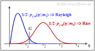
Density functions for "OOK, non-coherent"

$\text{Example 1:}$ The graph shows the result of this equation for $\sigma_n = 0.5$ and $C = 2$, where the (red) Rice PDF is approximated by a Gaussian PDF with mean $C$ and standard deviation $\sigma_n$.

One can see from this sketch:

The optimal decision value $($here: $G \approx 1.25)$ results from the intersection of the two PDF curves.

The symbol error probability $p_{\rm S}$ is the sum of the two colored areas. In the example: $p_{\rm S} \approx 5\%$ results.

⇒ You can determine the error probability for other values of $C$ and $\sigma_n$ as well as the optimal decision value $G$ using the (German language) SWF applet "Non-coherent On-Off Keying".

Non-coherent demodulation of binary FSK (2–FSK)

As already shown in the "last chapter", "Binary Frequency Shift Keying" $\rm (2–FSK)$ in the equivalent low-pass range can be described by the basis functions

\[\xi_1(t) = \sqrt{1/T} \cdot {\rm e}^{\hspace{0.05cm}+{\rm j} \hspace{0.03cm}\cdot \hspace{0.03cm} \pi \hspace{0.03cm}\cdot \hspace{0.03cm} h \hspace{0.03cm}\cdot \hspace{0.03cm}t/T}\hspace{0.05cm},\hspace{0.2cm} 0 \le t \le T\hspace{0.05cm},\]

\[ \xi_2(t) = \sqrt{1/T} \cdot {\rm e}^{\hspace{0.05cm}-{\rm j} \hspace{0.03cm}\cdot \hspace{0.03cm} \pi \hspace{0.03cm}\cdot \hspace{0.03cm} h \hspace{0.03cm}\cdot \hspace{0.03cm}t/T}\hspace{0.05cm},\hspace{0.2cm} 0 \le t \le T \hspace{0.05cm}\]

To achieve orthogonality between these two complex basis functions, the "modulation index" $h$ must be chosen to be integer:

\[< \hspace{-0.05cm}\xi_1(t) \hspace{0.1cm} \cdot \hspace{0.1cm} \xi_2(t) \hspace{-0.05cm}> \hspace{0.2cm}= 0 \hspace{0.3cm} \Rightarrow \hspace{0.3cm} h = 2 \cdot \Delta f_{\rm A} \cdot T\hspace{0.05cm}= 1, 2, 3, \text{...}\]

The diagram shows the structure for non-coherent orthogonal demodulation of binary FSK.

Non-coherent demodulation of the binary FSK

In the noise-free case ⇒ $n(t) \equiv 0$ applies to the outputs of the two correlators:

\[r_1 = \hspace{0.2cm} < \hspace{-0.05cm}r(t) \hspace{0.1cm} \cdot \hspace{0.1cm} \xi_1(t) \hspace{-0.05cm}> \hspace{0.2cm}= 0\hspace{0.05cm}, \hspace{0.4cm} {\rm if}\hspace{0.15cm} m = m_1\hspace{0.05cm},\]

\[ r_2 = \hspace{0.2cm} < \hspace{-0.05cm}r(t) \hspace{0.1cm} \cdot \hspace{0.1cm} \xi_2(t) \hspace{-0.05cm}> \hspace{0.2cm}= 0\hspace{0.05cm}, \hspace{0.4cm} {\rm if}\hspace{0.15cm} m = m_0\hspace{0.05cm}.\]

After respective magnitude formation ⇒ $y_1 = |r_1|, \ \ y_2 = |r_2|$ the following decision rule is applicable:

\[\hat{m} = \left\{ \begin{array}{c} m_0 \\ m_1 \end{array} \right.\quad \begin{array}{*{1}c} {\rm if}\hspace{0.15cm} y_1 > y_2 \hspace{0.05cm}, \\ {\rm if}\hspace{0.15cm} y_1 < y_2 \hspace{0.05cm}.\\ \end{array}\]

For a simpler realization of the decision, the difference $y_1 - y_2$ can also be evaluated with the decision boundary $G = 0$.

Error probability with non-coherent 2–FSK demodulation

In the following, the error probability is calculated under the assumption that $m = m_0$ was sent.

Under the further assumption of equally probable binary messages $m_0$ and $m_1$, the absolute error probability is exactly the same:

$${\rm Pr}({\cal{E}}) = {\rm Pr}({\cal{E}}\hspace{0.05cm} | \hspace{0.05cm}m_0) \hspace{0.05cm}.$$

With $m = m_0$ we get for the complex correlation output values $r_i$ and their magnitudes $y_i$:

\[r_1 = \sqrt{E} \cdot {\rm e}^{{\rm j}\phi} + n_1\hspace{0.3cm} \Rightarrow \hspace{0.3cm}y_1 = |r_1|\hspace{0.15cm}{\rm is}\hspace{0.15cm}{\rm Rice}\hspace{0.15cm}{\rm distributed} \hspace{0.05cm},\]

\[ r_2 = n_2\hspace{0.3cm} \Rightarrow \hspace{0.3cm}y_2 = |r_2|\hspace{0.15cm}{\rm is}\hspace{0.15cm}{\rm Rayleigh}\hspace{0.15cm}{\rm distributed} \hspace{0.05cm}.\]

Here, $E$ due to $M = 2$ represents the "average symbol energy" $(E_{\rm S})$ and the "average bit energy" $(E_{\rm B})$ equally. $n_1$ and $n_2$ are uncorrelated complex noise variables with mean zero and variance $2 \cdot \sigma_n^2$.

Thus, the "joint probability density function" is:

\[p_{y_1,\hspace{0.03cm} y_2 \hspace{0.03cm}| \hspace{0.03cm}m} ( \eta_1, \eta_2 \hspace{0.05cm}| \hspace{0.05cm}m_0) = p_{y_1 \hspace{0.01cm}| \hspace{0.03cm}m} ( \eta_1 \hspace{0.05cm}| \hspace{0.05cm}m_0) \cdot p_{y_2 \hspace{0.03cm}| \hspace{0.03cm}m} ( \eta_2 \hspace{0.05cm}| \hspace{0.05cm}m_0) \hspace{0.05cm},\]

$$p_{y_1 \hspace{0.01cm}| \hspace{0.03cm}m} ( \eta_1 \hspace{0.05cm}| \hspace{0.05cm}m_0) = {\eta_1}/{\sigma_n^2} \cdot {\rm e }^{ - ({\eta_1^2 + E})/({2 \sigma_n^2}) }\cdot {\rm I }_0 \left [{\eta_1 \cdot \sqrt{E}}/{ \sigma_n^2}\right ] \hspace{0.05cm},$$

$$ p_{y_2 \hspace{0.01cm}| \hspace{0.03cm}m} ( \eta_2 \hspace{0.05cm}| \hspace{0.05cm}m_0) = {\eta_2}/{\sigma_n^2} \cdot {\rm e }^{ - \eta_2^2 /({2 \sigma_n^2}) } \hspace{0.05cm}.$$

The error probability is generally obtained as follows:

\[{\rm Pr}({\cal{E}}) = \int_{0}^{\infty} \int_{\eta_1}^{\infty} p_{y_1,\hspace{0.03cm} y_2 \hspace{0.03cm}| \hspace{0.03cm}m} ( \eta_1, \eta_2 \hspace{0.05cm}| \hspace{0.05cm}m_0) \,\,{\rm d} \eta_2\,\,{\rm d} \eta_1 = \int_{0}^{\infty} p_{y_1 \hspace{0.01cm}| \hspace{0.03cm}m} ( \eta_1 \hspace{0.05cm}| \hspace{0.05cm}m_0) \cdot \int_{\eta_1}^{\infty} p_{y_2 \hspace{0.03cm}| \hspace{0.03cm}m} ( \eta_2 \hspace{0.05cm}| \hspace{0.05cm}m_0)\,\,{\rm d} \eta_2\,\,{\rm d} \eta_1 \hspace{0.05cm}.\]

$\text{Conclusion:}$ For the error probability with non-coherent demodulation of the binary FSK, one obtains after some mathematical transformations the surprisingly simple result

\[p_{\rm S} = {\rm Pr}({\cal{E} }) = {1}/{2} \cdot {\rm e}^{-E_{\rm S}/(2 N_0)} \hspace{0.05cm}.\]

For comparison, the result for coherent demodulation is here given again:

\[p_{\rm S} = {\rm Pr}({\cal{E} }) = {\rm Q}(\sqrt{ E_{\rm S}/N_0}) \hspace{0.05cm}.\]

$\text{Derivation:}$ This result is now to be derived in some calculation steps. We start from the following equations:

$${\rm Pr}({\cal{E} }) = \int_{0}^{\infty} p_{y_1 \hspace{0.01cm} \vert\hspace{0.03cm}m} ( \eta_1 \hspace{0.05cm} \vert \hspace{0.05cm}m_0) \cdot \int_{\eta_1}^{\infty} p_{y_2 \hspace{0.03cm}\vert \hspace{0.03cm}m} ( \eta_2 \hspace{0.05cm}\vert \hspace{0.05cm}m_0)\,\,{\rm d} \eta_2\,\,{\rm d} \eta_1 \hspace{0.05cm},\hspace{0.5cm}\text{with}$$

$$p_{y_1 \hspace{0.01cm}\vert \hspace{0.03cm}m} ( \eta_1 \hspace{0.05cm}\vert \hspace{0.05cm}m_0) = {\eta_1}/{\sigma_n^2} \cdot {\rm e }^{ - ({\eta_1^2 + E})/({2 \sigma_n^2}) }\cdot {\rm I }_0 \left [{\eta_1 \cdot \sqrt{E} }/{ \sigma_n^2}\right ] \hspace{0.05cm},$$

$$p_{y_\hspace{0.01cm}\vert \hspace{0.03cm}m} ( \eta_2 \hspace{0.05cm}\vert \hspace{0.05cm}m_0) = {\eta_2}/{\sigma_n^2} \cdot {\rm e }^{ - \eta_2^2 /({2 \sigma_n^2}) } \hspace{0.05cm}.$$

(1) The inner integral gives the probability that the Rayleigh distributed random variable $\eta_2$ is larger than $\eta_1$ – see solution to "Exercise 4.17Z":

$$\int_{\eta_1}^{\infty} p_{y_2 \hspace{0.03cm}\vert\hspace{0.03cm}m} ( \eta_2 \hspace{0.05cm}\vert \hspace{0.05cm}m_0)\,\,{\rm d} \eta_2 = {\rm e }^{ - \eta_1^2 /({2 \sigma_n^2}) } \hspace{0.3cm} \Rightarrow \hspace{0.3cm} {\rm Pr}({\cal{E} }) = \int_{0}^{\infty}{\eta_1}/{\sigma_n^2} \cdot {\rm e }^{ - ({2\eta_1^2 + E})/({2 \sigma_n^2}) }\cdot {\rm I }_0 \left [ {\eta_1 \cdot \sqrt{E} }/{ \sigma_n^2}\right ]\,\,{\rm d} \eta_1 \hspace{0.05cm}.$$

(2) With the (arbitrary) substitutions $C_0^2 = E/4$ and $\sigma_0^2 = \sigma_n^2/2$, we obtain:

$${\rm Pr}({\cal{E} }) = \int_{0}^{\infty} \frac{\eta_1}{2 \cdot \sigma_0^2} \cdot {\rm exp } \left [ - \frac{2 \eta_1^2 + 4 C_0^2}{4 \sigma_0^2}\right ] \cdot {\rm I }_0 \left [ \frac{\eta_1 \cdot 2C_0}{ 2 \sigma_0^2}\right ]\,\,{\rm d} \eta_1 = \int_{0}^{\infty} \frac{\eta_1}{2 \cdot \sigma_0^2} \cdot {\rm exp } \left [ - \frac{\eta_1^2 + 2 C_0^2}{2 \sigma_0^2}\right ] \cdot {\rm I }_0 \left [ \frac{\eta_1 \cdot C_0}{ \sigma_0^2}\right ]\,\,{\rm d} \eta_1 \hspace{0.05cm}.$$

(3) By shifting fractions in front of the integral, we succeed that the integrand again describes a "Rice distribution":

\[{\rm Pr}({\cal{E} }) = {1}/{2} \cdot {\rm exp } \left [ - \frac{ C_0^2}{2 \sigma_0^2}\right ] \cdot \int\limits_{0}^{\infty} \frac{\eta_1}{ \sigma_0^2} \cdot {\rm exp } \left [ - \frac{\eta_1^2 + C_0^2}{2 \sigma_0^2}\right ] \cdot {\rm I }_0 \left [ \frac{\eta_1 \cdot C_0}{ \sigma_0^2}\right ]\,\,{\rm d} \eta_1 \hspace{0.05cm}.\]

(4) The integrand now describes the Rice PDF. The integral over the entire definition area from $0$ to $+\infty$ yields the value one, as for any PDF, so that holds:

\[{\rm Pr}({\cal{E} }) = {1}/{2} \cdot {\rm exp } \left [ - \frac{ C_0^2}{2 \sigma_0^2}\right ]\hspace{0.05cm}.\]

(5) Finally, with $C_0^2 = E/4$ and $\sigma_0^2 = \sigma_n^2/2$ and the generally valid relation $\sigma_n^2 = N_0$, we obtain:

$${\rm Pr}({\cal{E} }) = {1}/{2} \cdot {\rm exp } \left [ - \frac{ C_0^2}{2 \sigma_0^2}\right ] = {1}/{2} \cdot {\rm exp } \left [ - \frac{ E_{\rm S}/4}{N_{\rm 0}/2}\right ] \hspace{0.3cm}\Rightarrow \hspace{0.3cm} p_{\rm S} = {\rm Pr}({\cal{E} }) = {1}/{2} \cdot {\rm e}^{-E_{\rm S}/(2 N_0)}\hspace{0.05cm}.$$

q.e.d. $E_{\rm S}$ here indicates the average signal energy per symbol, which is equal to the normalization energy $E$ for FSK.

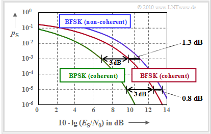
FSK symbol error probability for coherent and non-coherent demodulation

$\text{Example 2:}$ The graph compares the error probability curves of both demodulation methods as a function of the AWGN quotient $E_{\rm S}/N_0$.

One can see:

The non-coherent FSK (red curve) requires a $0.8 \ \rm dB$ larger $E_{\rm S}/N_0$ compared to the coherent FSK (blue curve) at $p_{\rm S}= 10^{-5}$.
At $p_{\rm S}= 10^{-3}$ the distance is even $1.3 \ \rm dB$.
In contrast, the distance between the coherent binary FSK from the coherent BPSK is always $1.3 \ \rm dB$ regardless of the error probability.

Non-coherent demodulation of multi-level FSK

Orthogonal $M$–level FSK for $M= 3$

We now consider the message set $\{m_1, m_2,\hspace{0.05cm}\text{ ...} \hspace{0.05cm}, m_{M}\}$ and denote $M$ as the "level number".

As in the case of binary FSK, a prerequisite for the application of the modulation process "Frequency Shift Keying" and at the same time of a non-coherent demodulator is an integer modulation index $h$.
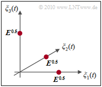
In this case, the $M$–level FSK is orthogonal and a signal space constellation results as shown in the adjacent diagram for the special case $M = 3$.

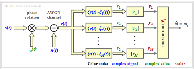
The non-coherent demodulator is sketched below.

Compared to the "receiver structure for binary FSK", this receiver differs only by $M$ branches instead of only two, which provide the comparison values $y_1$, $y_2$, ... , $y_M$.

To calculate the error probability, we assume that $m_1$ was sent. This means that the decision is correct if the largest detection output value is $y_1$:

\[{\rm Pr}({\cal{C}}) \hspace{-0.1cm} = \hspace{-0.1cm} {\rm Pr} \big [ (y_2 < y_1) \cap (y_3 < y_1) \cap ... \cap (y_{M} < y_1) \hspace{0.05cm}| \hspace{0.05cm} m = m_1\big ] = {\rm Pr} \left [ \hspace{0.1cm} \bigcap\limits_{k = 2}^M (y_k < y_1) \hspace{0.05cm}| \hspace{0.05cm}m = m_1\right ] \hspace{0.01cm}.\]

Non-coherent receiver structure for $M$–level FSK

$\text{Conclusions:}$

The error probability of M–level FSK in non-coherent demodulation is equal to ${\rm Pr}({\cal{E} }) = 1 - {\rm Pr}({\cal{C} })$.

In the following, it is shown that ${\rm Pr}({\cal{C} })$ can be represented as follows:

\[{\rm Pr}({\cal{C} }) = \sum_{i = 0}^{M-1} (-1)^i \cdot {M-1 \choose i } \cdot \frac{1}{i+1} \cdot {\rm exp } \left [ - \frac{i \cdot E_{\rm S} } {(i+1) \cdot N_0}\right ] \hspace{0.05cm}\hspace{0.5cm} \text{with}\hspace{0.5cm} E_{\rm S} = E_{\rm B} \cdot {\rm log_2}(M)\hspace{0.05cm}.\]

In the special case $M = 2$, of course, the result obtained in the "last section" is again obtained:

\[p_{\rm S} = {\rm Pr}({\cal{E} }) = {1}/{2} \cdot {\rm e}^{-E_{\rm S}/(2 N_0)} \hspace{0.05cm}.\]

$\text{Derivation:}$ This result shall now be derived in some calculation steps.

We assume that $m_1$ has been sent. This means that the decision is correct if the largest detection output value is $y_1$.

Otherwise, there are certain analogies to the derivation of the "BFSK error probability".

(1) Using the conditional probability density $p_{y_1 \hspace{0.01cm} \vert\hspace{0.03cm}m} ( \eta_1 \hspace{0.05cm} \vert \hspace{0.05cm}m_1)$, we obtain:

\[{\rm Pr}({\cal{C} }) = \int_{0}^{\infty} {\rm Pr} \left [ \hspace{0.1cm} \bigcap\limits_{k = 2}^M (y_k < y_1) \hspace{0.05cm}\vert\hspace{0.05cm}y_1 = \eta_1, m = m_1\right ] \cdot p_{y_1 \hspace{0.01cm} \vert\hspace{0.03cm}m} ( \eta_1 \hspace{0.05cm} \vert \hspace{0.05cm}m_1) \,\,{\rm d} \eta_1 \hspace{0.05cm}.\]

(2) The decision values $y_2$, $y_3$, ... , $y_M$ are statistically independent for given $y_1$. Therefore:

\[{\rm Pr}({\cal{C} }) = \int_{0}^{\infty} \left \{ {\rm Pr} \big [ (y_2 < y_1) \hspace{0.05cm}\vert \hspace{0.05cm}y_1 = \eta_1, m = m_1\big ] \right \}^{M-1} \cdot p_{y_1 \hspace{0.01cm} \vert\hspace{0.03cm}m} ( \eta_1 \hspace{0.05cm} \vert \hspace{0.05cm}m_1) \,\,{\rm d} \eta_1 \hspace{0.05cm}.\]

(3) The selected value $y_2$ conditioned on $m_1$ has a Rayleigh distribution with parameter $\sigma_n^2$:

\[{\rm Pr} \big [ (y_2 < y_1) \hspace{0.05cm} \vert \hspace{0.05cm}y_1 = \eta_1, m = m_1\big ] \hspace{-0.1cm} = \hspace{-0.1cm} \int_{0}^{\eta_1} p_{y_2 \hspace{0.01cm} \vert\hspace{0.03cm}m} ( \eta_2 \hspace{0.05cm} \vert \hspace{0.05cm}m_1)\,\,{\rm d} \eta_2= 1 - {\rm exp } \big [ - {\eta_1^2 }/({2 \sigma_n^2})\big ] = 1 - a \hspace{0.2cm}{\rm(abbreviation)} \hspace{0.05cm}.\]

(4) Now we are looking for the expression $(1 -a)^{M-1}$, for which with the abbreviation from (3) holds:

\[ (1-a)^{M-1} \hspace{-0.1cm} = \hspace{-0.1cm} \sum_{i = 0}^{M-1} (-1)^i \cdot {M-1 \choose i } \cdot (-1)^i \cdot a^i = \sum_{i = 0}^{M-1} (-1)^i \cdot {M-1 \choose i } \cdot {\rm exp } \left [ - \frac{i \cdot \eta_1^2 }{2 \sigma_n^2}\right ] \hspace{0.05cm}.\]

(5) $y_1$ has a "Rice distribution" conditioned on $m=m_1$. Thus, the probability of a correct decision can be expressed in the following form:

\[{\rm Pr}({\cal{C} }) \hspace{-0.1cm} = \hspace{-0.1cm} \sum_{i = 0}^{M-1} (-1)^i \cdot {M-1 \choose i } \cdot \int_{0}^{\infty} {\rm exp } \left [ - \frac{i \cdot \eta_1^2 }{2 \sigma_n^2}\right ] \cdot \frac{\eta_1}{ \sigma_n^2}\cdot {\rm exp } \left [ - \frac{\eta_1^2 + E_{\rm S} }{2 \sigma_n^2}\right ] \cdot {\rm I }_0 \left [ \frac{\eta_1 \cdot \sqrt{E_{\rm S} } }{ \sigma_n^2}\right ] \,\,{\rm d} \eta_1 \hspace{0.05cm}.\]

(6) Substitutions succeed in shaping the integrand according to the Rice distribution. Since each probability density integrates to one, we obtain:

\[{\rm Pr}({\cal{C} }) = \sum_{i = 0}^{M-1} (-1)^i \cdot {M-1 \choose i } \cdot \frac{1}{i+1} \cdot {\rm exp } \left [ - \frac{i \cdot E_{\rm S} } {(i+1) \cdot N_0}\right ] \hspace{0.05cm}\hspace{0.5cm} \text{with}\hspace{0.5cm} E_{\rm S} = E_{\rm B} \cdot {\rm log_2}(M)\hspace{0.05cm}.\]

(7) The special case $M = 2$ leads to exactly the same result as calculated for the binary FSK:

\[{\rm Pr}({\cal{C} }) = (-1)^0 \cdot {2-1 \choose 0 } \cdot \frac{1}{0+1} \cdot {\rm exp } \left [ - \frac{0 \cdot E_{\rm S} } {(i+1) \cdot N_0}\right ] + (-1)^1 \cdot {2-1 \choose 1 } \cdot \frac{1}{1+1} \cdot {\rm exp } \left [ - \frac{1 \cdot E_{\rm S} } {(i+1) \cdot N_0}\right ] \]

\[ \Rightarrow \hspace{0.5cm} {\rm Pr}({\cal{C} }) = 1 - {1}/{2} \cdot {\rm e }^{-E_{\rm S}/(2N_0)} \hspace{0.5cm} \Rightarrow \hspace{0.5cm} {\rm Pr}({\cal{E} }) = 1 - {\rm Pr}({\cal{C} }) = {1}/{2} \cdot {\rm e }^{-E_{\rm S}/(2N_0)} \hspace{0.05cm}.\]

Exercises for the chapter

Exercise 4.17: Non-Coherent On-Off Keying

Exercise 4.17Z: Rayleigh and Rice Distribution

Exercise 4.18: Non-Coherent FSK Demodulation

Exercise 4.18Z: BER of Coherent and Non-Coherent FSK

Exercise 4.19: Orthogonal Multilevel FSK