Exercise 3.10: Metric Calculation

Only partially evaluated trellis

In the "theory section" of this chapter, the calculation of the branch metrics ${\it \Gamma}_i(S_{\mu})$ has been discussed in detail, based on the Hamming distance $d_{\rm H}(\underline{x}\hspace{0.05cm}', \ \underline{y}_i)$ between the possible code words $\underline{x}\hspace{0.05cm}' ∈ \{00, \, 01, \, 10, \, 11\}$ and the 2–bit–words $\underline{y}_i$ received at time $i$ is based.

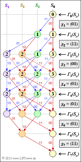
The exercise deals exactly with this topic. In the adjacent graph

the considered trellis is shown– valid for the code with rate $R = 1/2$, memory $m = 2$ and $\mathbf{G}(D) = (1 + D + D^2, \ 1 + D^2)$,
are the received words $\underline{y}_1 = (01), \hspace{0.05cm}\text{ ...} \hspace{0.05cm} , \ \underline{y}_7 = (11)$ indicated in the rectangles,
are all branch metrics ${\it \Gamma}_0(S_{\mu}), \hspace{0.05cm}\text{ ...} \hspace{0.05cm} , \ {\it \Gamma}_4(S_{\mu})$ already entered.

For example, the branch metric ${\it \Gamma}_4(S_0)$ with $\underline{y}_4 = (01)$ as the minimum of the two comparison values

${\it \Gamma}_3(S_0) + d_{\rm H}((00), \ (01)) = 3 + 1 = 4$, and
${\it \Gamma}_3(S_2) + d_{\rm H}((11), \ (01)) = 2 + 1 = 3$.

The surviving branch – here from ${\it \Gamma}_3(S_2)$ to ${\it \Gamma}_4(S_0)$ – is drawn solid, the eliminated branch from ${\it \Gamma}_3(S_0)$ to ${\it \Gamma}_4(S_0)$ dotted. Red arrows represent the information bit $u_i = 0$, blue arrows $u_i = 1$.

In the subtask (4) the relationship between

the ${\it \Gamma}_i(S_{\mu})$ minimization and
the ${\it \Lambda}_i(S_{\mu})$ maximization.

shall be worked out. Here, we refer to the nodes ${\it \Lambda}_i(S_{\mu})$ as metrics, where the metric increment over the predecessor nodes results from the correlation value $〈\underline{x}_i\hspace{0.05cm}', \, \underline{y}_i 〉$ . For more details on this topic, see the following theory pages:

Hints:

The exercise refers to the chapter "Decoding Convolutional Codes".
For the time being, the search of surviving paths is not considered. This will be dealt with for the same example in the later "Exercise 3.11".

Questions

${\it \Gamma}_5(S_0) \ = \ $

${\it \Gamma}_5(S_1) \ = \ $

${\it \Gamma}_5(S_2) \ = \ $

${\it \Gamma}_5(S_3) \ = \ $

${\it \Gamma}_6(S_0) \ = \ $

${\it \Gamma}_6(S_2) \ = \ $

	It holds ${\it \Gamma}_7(S_0) = 3$.
	This final value suggests one error-free transmission.
	This final value suggests three transmission errors.

	The metrics ${\it \Lambda}_i(S_{\mu})$ provide the same information as ${\it \Gamma}_i(S_{\mu})$.
	For all nodes, ${\it \Lambda}_i(S_{\mu}) = 2 \cdot \big [i \, –{\it \Gamma}_i(S_{\mu})\big ]$.
	For the metric increments, $〈 \underline{x}_i', \, \underline{y}_i 〉 ∈ \{0, \, 1, \, 2\}$.

Solution

(1) At all nodes $S_{\mu}$ a decision must be made between the two incoming branches. The branch that led to the (minimum) error metric ${\it \Gamma}_5(S_{\mu})$ is then selected in each case. With $\underline{y}_5 = (01)$ one obtains:

$${\it \Gamma}_5(S_0) \hspace{-0.15cm} \ = \ \hspace{-0.15cm}{\rm min} \left [{\it \Gamma}_{4}(S_0) + d_{\rm H} \big ((00)\hspace{0.05cm},\hspace{0.05cm} (01) \big )\hspace{0.05cm},\hspace{0.2cm}{\it \Gamma}_{4}(S_2) + d_{\rm H} \big ((11)\hspace{0.05cm},\hspace{0.05cm} (01) \big ) \right ] ={\rm min} \left [ 3+1\hspace{0.05cm},\hspace{0.05cm} 2+1 \right ] \hspace{0.15cm}\underline{= 3}\hspace{0.05cm},$$

$${\it \Gamma}_5(S_1) \hspace{-0.15cm} \ = \ \hspace{-0.15cm}{\rm min} \left [{\it \Gamma}_{4}(S_0) + d_{\rm H} \big ((11)\hspace{0.05cm},\hspace{0.05cm} (01) \big )\hspace{0.05cm},\hspace{0.2cm}{\it \Gamma}_{4}(S_2) + d_{\rm H} \big ((00)\hspace{0.05cm},\hspace{0.05cm} (01) \big ) \right ] ={\rm min} \left [ 3+1\hspace{0.05cm},\hspace{0.05cm} 2+1 \right ] \hspace{0.15cm}\underline{= 3}\hspace{0.05cm},$$

$${\it \Gamma}_5(S_2) \hspace{-0.15cm} \ = \ \hspace{-0.15cm}{\rm min} \left [{\it \Gamma}_{4}(S_1) + d_{\rm H} \big ((10)\hspace{0.05cm},\hspace{0.05cm} (01) \big )\hspace{0.05cm},\hspace{0.2cm}{\it \Gamma}_{4}(S_3) + d_{\rm H} \big ((01)\hspace{0.05cm},\hspace{0.05cm} (01) \big ) \right ] = {\rm min} \left [ 3+2\hspace{0.05cm},\hspace{0.05cm} 2+0 \right ] \hspace{0.15cm}\underline{= 2}\hspace{0.05cm},$$

$${\it \Gamma}_5(S_3) \hspace{-0.15cm} \ = \ \hspace{-0.15cm}{\rm min} \left [{\it \Gamma}_{4}(S_1) + d_{\rm H} \big ((01)\hspace{0.05cm},\hspace{0.05cm} (01) \big )\hspace{0.05cm},\hspace{0.2cm}{\it \Gamma}_{4}(S_3) + d_{\rm H} \big ((10)\hspace{0.05cm},\hspace{0.05cm} (01) \big ) \right ] ={\rm min} \left [ 3+0\hspace{0.05cm},\hspace{0.05cm} 2+2 \right ] \hspace{0.15cm}\underline{= 3}\hspace{0.05cm}.$$

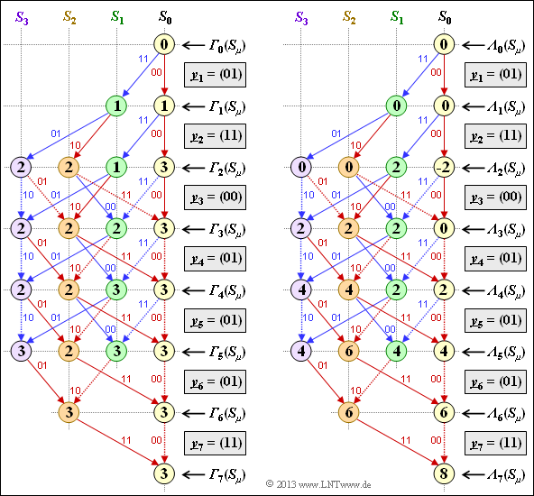
The left graph shows the final evaluated ${\it \Gamma}_i(S_{\mu})$ trellis.

Evaluated trellis diagrams

(2) At time $i = 6$ the termination is already effective and there are only two branch metrics left. For these one obtains with $\underline{y}_6 = (01)$:

$${\it \Gamma}_6(S_0) \hspace{-0.15cm} \ = \ \hspace{-0.15cm}{\rm min} \left [{\it \Gamma}_{5}(S_0) + d_{\rm H} \big ((00)\hspace{0.05cm},\hspace{0.05cm} (01) \big )\hspace{0.05cm},\hspace{0.2cm}{\it \Gamma}_{5}(S_2) + d_{\rm H} \big ((11)\hspace{0.05cm},\hspace{0.05cm} (01) \big ) \right ] ={\rm min} \left [ 3+1\hspace{0.05cm},\hspace{0.05cm} 2+1 \right ] \hspace{0.15cm}\underline{= 3}\hspace{0.05cm},$$

$${\it \Gamma}_6(S_2) \hspace{-0.15cm} \ = \ \hspace{-0.15cm}{\rm min} \left [{\it \Gamma}_{5}(S_1) + d_{\rm H} \big ((10)\hspace{0.05cm},\hspace{0.05cm} (01) \big )\hspace{0.05cm},\hspace{0.2cm}{\it \Gamma}_{5}(S_3) + d_{\rm H} \big ((01)\hspace{0.05cm},\hspace{0.05cm} (01) \big ) \right ] ={\rm min} \left [ 3+2\hspace{0.05cm},\hspace{0.05cm} 3+0 \right ] \hspace{0.15cm}\underline{= 3}\hspace{0.05cm}.$$

(3) The final value results to

$${\it \Gamma}_7(S_0) \hspace{-0.15cm} \ = \ \hspace{-0.15cm}{\rm min} \left [{\it \Gamma}_{6}(S_0) + d_{\rm H} \big ((00)\hspace{0.05cm},\hspace{0.05cm} (11) \big )\hspace{0.05cm},\hspace{0.2cm}{\it \Gamma}_{6}(S_2) + d_{\rm H} \big ((11)\hspace{0.05cm},\hspace{0.05cm} (11) \big ) \right ] ={\rm min} \left [ 3+2\hspace{0.05cm},\hspace{0.05cm} 3+0 \right ] \hspace{0.15cm}\underline{= 3}\hspace{0.05cm}.$$

In the BSC model, one can infer from ${\it \Gamma}_7(S_{\mu}) = 3$ that three transmission errors occurred ⇒ solutions 1 and 3.

(4) Correct are statements 1 and 2:

Maximizing the branch metrics ${\it \Lambda}_i(S_{\mu})$ according to the right sketch in the above graph gives the same result as minimizing the branch metrics ${\it \Gamma}_i(S_{\mu})$ shown on the left. Also, the surviving and deleted branches are identical in both graphs.
The given equation is also correct, which is shown here only on the example $i = 7$:

$${\it \Lambda}_7(S_0)) = 2 \cdot \big [i - {\it \Gamma}_7(S_0) \big ] = 2 \cdot \big [7 - 3 \big ] \hspace{0.15cm}\underline{= 8}\hspace{0.05cm}.$$

The last statement is false. Rather applies $〈x_i', \, y_i〉 ∈ \{–2, \, 0, \, +2\}$.

Hints: In "Exercise 3.11", path finding is demonstrable for the same example, assuming ${\it \Lambda}_i(S_{\mu})$–metrics as shown in the right graph.