Two-dimensional Gaussian Random Variables

Open Applet in new Tab Deutsche Version Öffnen

Applet Description

The applet illustrates the properties of two-dimensional Gaussian random variables $XY\hspace{-0.1cm}$, characterized by the standard deviations (rms) $\sigma_X$ and $\sigma_Y$ of their two components, and the correlation coefficient $\rho_{XY}$ between them. The components are assumed to be zero mean: $m_X = m_Y = 0$.

The applet shows

the two-dimensional probability density function ⇒ $\rm 2D\hspace{-0.1cm}-\hspace{-0.1cm}PDF$ $f_{XY}(x, \hspace{0.1cm}y)$ in three-dimensional representation as well as in the form of contour lines,
the corresponding marginal probability density function ⇒ $\rm 1D\hspace{-0.1cm}-\hspace{-0.1cm}PDF$ $f_{X}(x)$ of the random variable $X$ as a blue curve; likewise $f_{Y}(y)$ for the second random variable,
the two-dimensional distribution function ⇒ $\rm 2D\hspace{-0.1cm}-\hspace{-0.1cm}CDF$ $F_{XY}(x, \hspace{0.1cm}y)$ as a 3D plot,
the distribution function ⇒ $\rm 1D\hspace{-0.1cm}-\hspace{-0.1cm}CDF$ $F_{X}(x)$ of the random variable $X$; also $F_{Y}(y)$ as a red curve.

The applet uses the framework Plot.ly

Theoretical Background

Joint probability density function ⇒ 2D–PDF

We consider two continuous value random variables $X$ and $Y\hspace{-0.1cm}$, between which statistical dependencies may exist. To describe the interrelationships between these variables, it is convenient to combine the two components into a two-dimensional random variable $XY =(X, Y)$ . Then holds:

$\text{Definition:}$ The joint probability density function is the probability density function (PDF) of the two-dimensional random variable $XY$ at location $(x, y)$:

$$f_{XY}(x, \hspace{0.1cm}y) = \lim_{\left.{\delta x\rightarrow 0 \atop {\delta y\rightarrow 0} }\right. }\frac{ {\rm Pr}\big [ (x - {\rm \Delta} x/{\rm 2} \le X \le x + {\rm \Delta} x/{\rm 2}) \cap (y - {\rm \Delta} y/{\rm 2} \le Y \le y +{\rm \Delta}y/{\rm 2}) \big] }{ {\rm \Delta} \ x\cdot{\rm \Delta} y}.$$

The joint probability density function, or in short $\rm 2D\hspace{-0.1cm}-\hspace{-0.1cm}PDF$ is an extension of the one-dimensional PDF.
$∩$ denotes the logical AND operation.
$X$ and $Y$ denote the two random variables, and $x \in X$ and $y \in Y$ indicate realizations thereof.
The nomenclature used for this applet thus differs slightly from the description in the Theory section.

Using this 2D–PDF $f_{XY}(x, y)$ statistical dependencies within the two-dimensional random variable $XY$ are also fully captured in contrast to the two one-dimensional density functions ⇒ marginal probability density functions:

$$f_{X}(x) = \int _{-\infty}^{+\infty} f_{XY}(x,y) \,\,{\rm d}y ,$$

$$f_{Y}(y) = \int_{-\infty}^{+\infty} f_{XY}(x,y) \,\,{\rm d}x .$$

These two marginal density functions $f_X(x)$ and $f_Y(y)$

provide only statistical information about the individual components $X$ and $Y$, respectively,
but not about the bindings between them.

As a quantitative measure of the linear statistical bindings ⇒ correlation one uses.

the covariance $\mu_{XY}$, which is equal to the first-order common linear moment for mean-free components:

$$\mu_{XY} = {\rm E}\big[X \cdot Y\big] = \int_{-\infty}^{+\infty} \int_{-\infty}^{+\infty} X \cdot Y \cdot f_{XY}(x,y) \,{\rm d}x \, {\rm d}y ,$$

the correlation coefficient after normalization to the two rms values $σ_X$ and $σ_Y$ of the two components:

$$\rho_{XY}=\frac{\mu_{XY} }{\sigma_X \cdot \sigma_Y}.$$

$\text{Properties of correlation coefficient:}$

Because of normalization, $-1 \le ρ_{XY} ≤ +1$ always holds .
If the two random variables $X$ and $Y$ are uncorrelated, then $ρ_{XY} = 0$.
For strict linear dependence between $X$ and $Y$, $ρ_{XY}= ±1$ ⇒ complete correlation.
A positive correlation coefficient means that when $X$ is larger, on statistical average, $Y$ is also larger than when $X$ is smaller.
In contrast, a negative correlation coefficient expresses that $Y$ becomes smaller on average as $X$ increases

.

2D–PDF for Gaussian random variables

For the special case Gaussian random variables - the name goes back to the scientist Carl Friedrich Gauss - we can further note:

The joint PDF of a Gaussian 2D random variable $XY$ with means $m_X = 0$ and $m_Y = 0$ and the correlation coefficient $ρ = ρ_{XY}$ is:

$$f_{XY}(x, y)=\frac{\rm 1}{\rm 2\it\pi \cdot \sigma_X \cdot \sigma_Y \cdot \sqrt{\rm 1-\rho^2}}\ \cdot\ \exp\Bigg[-\frac{\rm 1}{\rm 2 \cdot (1- \it\rho^{\rm 2} {\rm)}}\cdot(\frac {\it x^{\rm 2}}{\sigma_X^{\rm 2}}+\frac {\it y^{\rm 2}}{\sigma_Y^{\rm 2}}-\rm 2\it\rho\cdot\frac{x \cdot y}{\sigma_x \cdot \sigma_Y}\rm ) \rm \Bigg]\hspace{0.8cm}{\rm with}\hspace{0.5cm}-1 \le \rho \le +1.$$

Replacing $x$ by $(x - m_X)$ and $y$ by $(y- m_Y)$, we obtain the more general PDF of a two-dimensional Gaussian random variable with mean.
The marginal probability density functions $f_{X}(x)$ and $f_{Y}(y)$ of a 2D Gaussian random variable are also Gaussian with the standard deviations $σ_X$ and $σ_Y$, respectively.
For uncorrelated components $X$ and $Y$, in the above equation $ρ = 0$ must be substituted, and then the result is obtained:

$$f_{XY}(x,y)=\frac{1}{\sqrt{2\pi}\cdot\sigma_{X}} \cdot\rm e^{-\it {x^{\rm 2}}\hspace{-0.08cm}/{\rm (}{\rm 2\hspace{0.05cm}\it\sigma_{X}^{\rm 2}} {\rm )}} \cdot\frac{1}{\sqrt{2\pi}\cdot\sigma_{\it Y}}\cdot e^{-\it {y^{\rm 2}}\hspace{-0.08cm}/{\rm (}{\rm 2\hspace{0.05cm}\it\sigma_{Y}^{\rm 2}} {\rm )}} = \it f_{X} \rm ( \it x \rm ) \cdot \it f_{Y} \rm ( \it y \rm ) .$$

$\text{Conclusion:}$ In the special case of a 2D random variable with Gaussian PDF $f_{XY}(x, y)$ it also follows directly from uncorrelatedness the statistical independence:

$$f_{XY}(x,y)= f_{X}(x) \cdot f_{Y}(y) . $$

Please note:

For no other PDF can the uncorrelatedness be used to infer statistical independence .
But one can always ⇒ infer uncorrelatedness from statistical independence for any 2D-PDF $f_{XY}(x, y)$ because:
If two random variables $X$ and $Y$ are completely (statistically) independent of each other, then of course there are no linear dependencies between them
⇒ they are then also uncorrelated ⇒ $ρ = 0$.

Contour lines for uncorrelated random variables

Contour lines of 2D-PDF with uncorrelated variables

From the conditional equation $f_{XY}(x, y) = {\rm const.}$ the contour lines of the PDF can be calculated.

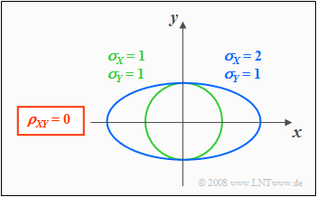
If the components $X$ and $Y$ are uncorrelated $(ρ_{XY} = 0)$, the equation obtained for the contour lines is:

$$\frac{x^{\rm 2}}{\sigma_{X}^{\rm 2}}+\frac{y^{\rm 2}}{\sigma_{Y}^{\rm 2}} =\rm const.$$

In this case, the contour lines describe the following figures:

Circles (if $σ_X = σ_Y$, green curve), or
Ellipses (for $σ_X ≠ σ_Y$, blue curve) in alignment of the two axes.

Regression line

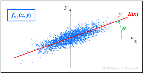
As regression line is called the straight line $y = K(x)$ in the $(x, y)$–plane through the "center" $(m_X, m_Y)$. This has the following properties:

Gaussian 2D PDF (approximation with $N$ measurement points) and
correlation line $y = K(x)$

The mean square error from this straight line - viewed in $y$–direction and averaged over all $N$ measurement points - is minimal:

$$\overline{\varepsilon_y^{\rm 2} }=\frac{\rm 1}{N} \cdot \sum_{\nu=\rm 1}^{N}\; \;\big [y_\nu - K(x_{\nu})\big ]^{\rm 2}={\rm minimum}.$$

The correlation straight line can be interpreted as a kind of "statistical symmetry axis". The equation of the straight line in the general case is:

$$y=K(x)=\frac{\sigma_Y}{\sigma_X}\cdot\rho_{XY}\cdot(x - m_X)+m_Y.$$

The angle that the correlation line makes to the $x$–axis is:

$$\theta={\rm arctan}(\frac{\sigma_{Y} }{\sigma_{X} }\cdot \rho_{XY}).$$

Contour lines for correlated random variables

For correlated components $(ρ_{XY} ≠ 0)$ the contour lines of the PDF are (almost) always elliptic, so also for the special case $σ_X = σ_Y$.

Exception: $ρ_{XY}=\pm 1$ ⇒ Diracwand; see Exercise 4.4 in the book "Stochastic Signal Theory", subtask (5)'.

height lines of the two dimensional PDF with correlated quantities

Here, the determining equation of the PDF height lines is:

$$f_{XY}(x, y) = {\rm const.} \hspace{0.5cm} \rightarrow \hspace{0.5cm} \frac{x^{\rm 2} }{\sigma_{X}^{\rm 2}}+\frac{y^{\rm 2} }{\sigma_{Y}^{\rm 2} }-{\rm 2}\cdot\rho_{XY}\cdot\frac{x\cdot y}{\sigma_X\cdot \sigma_Y}={\rm const.}$$

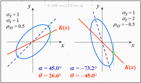
The graph shows a contour line in lighter blue for each of two different sets of parameters.

The ellipse major axis is dashed in dark blue.
The regression line $K(x)$ is drawn in red throughout.

Based on this plot, the following statements are possible:

The ellipse shape depends not only on the correlation coefficient $ρ_{XY}$ but also on the ratio of the two standard deviations $σ_X$ and $σ_Y$ .
The angle of inclination $α$ of the ellipse major axis (dashed straight line) with respect to the $x$–axis also depends on $σ_X$, $σ_Y$ and $ρ_{XY}$ :

$$\alpha = {1}/{2} \cdot {\rm arctan } \big ( 2 \cdot \rho_{XY} \cdot \frac {\sigma_X \cdot \sigma_Y}{\sigma_X^2 - \sigma_Y^2} \big ).$$

The (red) correlation line $y = K(x)$ of a Gaussian 2D random variable always lies below the (blue dashed) ellipse major axis.
$K(x)$ can be geometrically constructed from the intersection of the contour lines and their vertical tangents, as indicated in the sketch in green color.

Two dimensional cumulative distribution function ⇒ 2D–CDF

$\text{Definition:}$ The 2D cumulative distribution function like the 2D-CDF, is merely a useful extension of the one-dimensional distribution function (PDF):

$$F_{XY}(x,y) = {\rm Pr}\big [(X \le x) \cap (Y \le y) \big ] .$$

The following similarities and differences between the "1D–CDF" and the" 2D–CDF" emerge:

The functional relationship between "2D–PDF" and "2D–CDF" is given by the integration as in the one-dimensional case, but now in two dimensions. For continuous random variables, the following holds:

$$F_{XY}(x,y)=\int_{-\infty}^{y} \int_{-\infty}^{x} f_{XY}(\xi,\eta) \,\,{\rm d}\xi \,\, {\rm d}\eta .$$

Inversely, the probability density function can be given from the cumulative distribution function by partial differentiation to $x$ and $y$ :

$$f_{XY}(x,y)=\frac{{\rm d}^{\rm 2} F_{XY}(\xi,\eta)}{{\rm d} \xi \,\, {\rm d} \eta}\Bigg|_{\left.{x=\xi \atop {y=\eta}}\right.}.$$

In terms of the cumulative distribution function $F_{XY}(x, y)$ the following limits apply:

$$F_{XY}(-\infty,\ -\infty) = 0,\hspace{0.5cm}F_{XY}(x,\ +\infty)=F_{X}(x ),\hspace{0.5cm} F_{XY}(+\infty,\ y)=F_{Y}(y ) ,\hspace{0.5cm}F_{XY}(+\infty,\ +\infty) = 1.$$

In the limiting case $($infinitely large $x$ and $y)$ thus the value $1$ is obtained for the "2D–CDF". From this we obtain the normalization condition for the two-dimensional probability density function:

$$\int_{-\infty}^{+\infty} \int_{-\infty}^{+\infty} f_{XY}(x,y) \,\,{\rm d}x \,\,{\rm d}y=1 . $$

$\text{Conclusion:}$ Note the significant difference between one-dimensional and two-dimensional random variables:

For one-dimensional random variables, the area under the PDF always yields $1$.
For two-dimensional random variables, the PDF volume always equals $1$.

Exercises

Select the number $(1,\ 2$, ... $)$ of the task to be processed. The number "0" corresponds to a "Reset": Setting as at the program start.
A task description is displayed. Parameter values are adjusted. Solution after pressing "Sample solution".
In the task description, we use $\rho$ instead of $\rho_{XY}$.
For the one-dimensional Gaussian PDF holds: $f_{X}(x) = \sqrt{1/(2\pi \cdot \sigma_X^2)} \cdot {\rm e}^{-x^2/(2 \hspace{0.05cm}\cdot \hspace{0.05cm} \sigma_X^2)}$.

(1) Get familiar with the program using the default $(\sigma_X=1, \ \sigma_Y=0.5, \ \rho = 0.7)$. Interpret the graphs for $\rm PDF$ and $\rm CDF$.

$\rm PDF$ is a ridge with the maximum at $x = 0, \ y = 0$. The ridge is slightly twisted with respect to the $x$–axis.
$\rm CDF$ is obtained from $\rm PDF$ by continuous integration in both directions. The maximum $($near $1)$ occurs at $x=3, \ y=3$.

(2) The new setting is $\sigma_X= \sigma_Y=1, \ \rho = 0$. What are the values for $f_{XY}(0,\ 0)$ and $F_{XY}(0,\ 0)$? Interpret the results

The PDF maximum is $f_{XY}(0,\ 0) = 1/(2\pi)= 0.1592$, because of $\sigma_X= \sigma_Y = 1, \ \rho = 0$. The contour lines are circles.
For the CDF value: $F_{XY}(0,\ 0) = [{\rm Pr}(X \le 0)] \cdot [{\rm Pr}(Y \le 0)] = 0.25$. Minor deviation due to numerical integration.

(3) The settings of $(2)$ continue to apply. What are the values for $f_{XY}(0,\ 1)$ and $F_{XY}(0,\ 1)$? Interpret the results.

It holds $f_{XY}(0,\ 1) = f_{X}(0) \cdot f_{Y}(1) = [ \sqrt{1/(2\pi)}] \cdot [\sqrt{1/(2\pi)} \cdot {\rm e}^{-0.5}] = 1/(2\pi) \cdot {\rm e}^{-0.5} = 0.0965$.
The program returns $F_{XY}(0,\ 1) = [{\rm Pr}(X \le 0)] \cdot [{\rm Pr}(Y \le 1)] = 0.4187$, i.e. a larger value than in $(2)$, since it integrates over a wider range.

(4) The settings are kept. What values are obtained for $f_{XY}(1,\ 0)$ and $F_{XY}(1,\ 0)$? Interpret the results

Due to rotational symmetry, same results as in $(3)$.

(5) Is the statement true: "Elliptic contour lines exist only for $\rho \ne 0$". Interpret the $\rm 2D\hspace{-0.1cm}-\hspace{-0.1cm}PDF$ and $\rm 2D\hspace{-0.1cm}-\hspace{-0.1cm}CDF$ for $\sigma_X=1, \ \sigma_Y=0.5$ and $\rho = 0$.

No! Also, for $\ \rho = 0$ the contour lines are elliptical (not circular) if $\sigma_X \ne \sigma_Y$.
For $\sigma_X \gg \sigma_Y$ the $\rm 2D\hspace{-0.1cm}-\hspace{-0.1cm}PDF$ has the shape of an elongated ridge parallel to $x$–axis, for $\sigma_X \ll \sigma_Y$ parallel to $y$–axis.
For $\sigma_X \gg \sigma_Y$ the slope of $\rm 2D\hspace{-0.1cm}-\hspace{-0.1cm}CDF$ in the direction of the $y$–axis is much steeper than in the direction of the $x$–axis.

(6) Starting from $\sigma_X=\sigma_Y=1\ \rho = 0.7$ vary the correlation coefficient $\rho$. What is the slope angle $\alpha$ of the ellipse main axis?

For $\rho > 0$: $\alpha = 45^\circ$. For $\rho < 0$: $\alpha = -45^\circ$. For $\rho = 0$: The contour lines are circular and thus there are no ellipses main axis.

(7) Starting from $\sigma_X=\sigma_Y=1\ \rho = 0.7$ vary the correlation coefficient $\rho$. What is the slope angle $\theta$ of the correlation line $K(x)$?

For $\sigma_X=\sigma_Y$&:nbsp; $\theta={\rm arctan}\ (\rho)$. The slope increases with increasing $\rho > 0$. In all cases, $\theta < \alpha = 45^\circ$ holds. For $\rho = 0.7$ this gives $\theta = 35^\circ$.

(8) Starting from $\sigma_X=\sigma_Y=0.75, \ \rho = 0.7$ vary the parameters $\sigma_Y$ and $\rho $. What statements hold for the angles $\alpha$ and $\theta$?

For $\sigma_Y<\sigma_X$: $\alpha < 45^\circ$. For $\sigma_Y>\sigma_X$: $\alpha > 45^\circ$. For all settings: The correlation line is below the ellipse main axis.

(9) Assume $\sigma_X= 1, \ \sigma_Y=0.75, \ \rho = 0.7$. Vary $\rho$. How to construct the correlation line from the contour lines?

The correlation line intersects all contour lines at that points where the tangent line is perpendicular to the contour line.

(10) Now let be $\sigma_X= \sigma_Y=1, \ \rho = 0.95$. Interpret the $\rm 2D\hspace{-0.1cm}-\hspace{-0.1cm}PDF$. Which statements are true for the limiting case $\rho \to 1$ ?

The $\rm 2D\hspace{-0.1cm}-\hspace{-0.1cm}WDF$ only has components near the ellipse main axis. The correlation line is just below: $\alpha = 45^\circ, \ \theta = 43.5^\circ$.
In the limiting case $\rho \to 1$ it holds $\theta = \alpha = 45^\circ$. Outside the correlation line, the $\rm 2D\hspace{-0.1cm}-\hspace{-0.1cm}PDF$ would have no shares. That is:
Along the correlation line, there would be a "Dirac wall" ⇒ All values are infinitely large, nevertheless Gaussian weighted around the mean.

Applet Manual

Screen shot (German version)

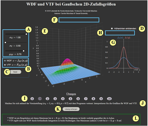
(A) Parametereingabe per Slider: $\sigma_X$, $\sigma_Y$ und $\rho$

(B) Auswahl: Darstellung von WDF oder VTF

(C) Reset: Einstellung wie beim Programmstart

(D) Höhenlinien darstellen anstelle von "1D-WDF"

(E) Darstellungsbereich für "2D-WDF"

(F) Manipulation der 3D-Grafik (Zoom, Drehen, ...)

(G) Darstellungsbereich für "1D-WDF" bzw. "Höhenlinien"

(H) Manipulation der 2D-Grafik ("1D-WDF")

( I ) Bereich für die Versuchsdurchführung: Aufgabenauswahl

(J) Bereich für die Versuchsdurchführung: Aufgabenstellung

(K) Bereich für die Versuchsdurchführung: Musterlösung einblenden

( L) Bereich für die Versuchsdurchführung: Musterlösung

Werte–Ausgabe über Maussteuerung (sowohl bei 2D als auch bei 3D)

About the Authors

This interactive calculation tool was designed and implemented at the Institute for Communications Engineering at the Technical University of Munich.

The first version was created in 2003 by Ji Li as part of his diploma thesis with “FlashMX – Actionscript” (Supervisor: Günter Söder).
In 2019 the program was redesigned by Carolin Mirschina as part of her bachelor thesis (Supervisor: Tasnád Kernetzky ) via "HTML5".
Last revision and English version 2021 by Carolin Mirschina in the context of a working student activity. Translation using DEEPL.com.

The conversion of this applet to HTML 5 was financially supported by "Studienzuschüsse" (Faculty EI of the TU Munich). We thank.

Once again: Open Applet in new Tab