Digital Filters

Open Applet in new Tab Deutsche Version Öffnen

Applet Description

The applet should clarify the properties of digital filters, whereby we confine ourselves to filters of the order $M=2$. Both non-recursive filters $\rm (FIR$, Finite Impulse Response$)$ as well as recursive filters $\rm (IIR$, Infinite Impulse Response$)$.

The input signal $x(t)$ is represented by the sequence $〈x_ν〉$ of its samples, where $x_ν$ stands for $x(ν · T_{\rm A})$. The output sequence $〈y_ν〉$is calculated, i.e. the discrete-time representation of the output signal $y(t)$.

$T_{\rm A}$ denotes the time interval between two samples.
We also limit ourselves to causal signals and systems, which means that $x_ν \equiv 0$ and $y_ν \equiv 0$ for $ν \le 0$.

It should also be noted that we denote the initial sequence $〈y_ν〉$ as

(1) the discrete-time impulse response $〈h_ν〉$ if the “discrete-time Dirac delta function” is present at the input: $〈x_ν〉= 〈1,\ 0,\ 0,\ 0,\ 0,\ 0,\ 0, \text{...}〉,$

(2) the discrete-time step response $〈\sigma_ν〉$ if the “discrete-time step function” is present at the input: $〈x_ν〉= 〈1,\ 1,\ 1,\ 1,\ 1,\ 1,\ 1, \text{...}〉,$

(3) the discrete-time rectangle response $〈\rho_ν^{(2, 4)}〉$ if the “discrete-time rectangle function” is present at the input: $〈x_ν〉= 〈0,\ 0,\ 1,\ 1,\ 1,\ 0,\ 0, \text{...}〉;$
In quotation marks are the beginning of the ones $(2)$ and the position of the last ones $(4)$.

Theoretical background

General block diagram

Each signal $x(t)$ can only be represented on a computer by the sequence $〈x_ν〉$ of its samples, where $x_ν$ stands for $x(ν · T_{\rm A})$.

Block diagram of a digital (IIR–) filter $M$–order

The time interval $T_{\rm A}$ between two samples is limited by the "sampling theorem".
We limit ourselves here to causal signals and systems, which means that $x_ν \equiv 0$ for $ν \le 0$.

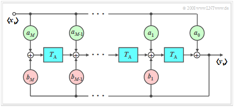
In order to determine the influence of a linear filter with frequency response $H(f)$ on the discrete-time input signal $〈x_ν〉$, it is advisable to describe the filter discrete-time. In the time domain, this happens with the discrete-time impulse response $〈h_ν〉$.
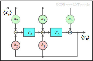
On the right you can see the corresponding block diagram. The following therefore applies to the samples of the output signal $〈y_ν〉$ thus holds:

$$y_\nu = \sum\limits_{\mu = 0}^M {a_\mu } \cdot x_{\nu - \mu } + \sum\limits_{\mu = 1}^M {b_\mu } \cdot y_{\nu - \mu } .$$

The following should be noted here:

The index $\nu$ refers to sequences, for example at the input $〈x_ν〉$ and output $〈y_ν〉$.
On the other hand, we use the index $\mu$ to identify the $a$ and $b$ filter coefficients.
The first sum describes the dependency of the current output $y_ν$ on the current input $x_ν$ and on the $M$ previous input values $x_{ν-1}$, ... , $x_{ν-M}$.
The second sum indicates the influence of $y_ν$ by the previous values $y_{ν-1}$, ... , $y_{ν-M}$ at the filter output. It specifies the recursive part of the filter.
The integer parameter $M$ is called the order of the digital filter. In the program, this value is limited to $M\le 2$.

$\text{Definitions:}$

(1) The output sequence $〈y_ν〉$ is called the discrete-time impulse response $〈h_ν〉$ if the “discrete-time Dirac delta function” is present at the input:

$$〈x_ν〉= 〈1,\ 0,\ 0,\ 0,\ 0,\ 0,\ 0, \text{...}〉 .$$

(2) The output sequence $〈y_ν〉$ is called the discrete-time step response $〈\sigma_ν〉$ if the “discrete-time step function” is present at the input:

$$〈x_ν〉= 〈1,\ 1,\ 1,\ 1,\ 1,\ 1,\ 1, \text{...}〉 .$$

(3) The output sequence $〈y_ν〉$ is called the discrete-time rectangle response $〈\rho_ν^{(2, 4)}〉$ if the “discrete-time rectangular function” is present at the input:

$$〈x_ν〉= 〈0,\ 0,\ 1,\ 1,\ 1,\ 0,\ 0, \text{...}〉 .$$

The beginning of ones $(2)$ and the position of the last ones $(4)$ are given in single quotes.

Non-recursive filter ⇒ FIR–filter

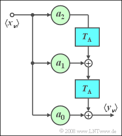
Non-recursive digital filter $($FIR filter$)$ $M$ order

$\text{Definition:}$ If all feedback coefficients $b_{\mu} = 0$ , one speaks of one non-recursive filter. In the English language literature, the term FIR filter (Finite Impulse Response) is also used for this.

The following applies to the order $M$ applies:

The output value $y_ν$ depends only on the current and the previous $M$ input values:

$$y_\nu = \sum\limits_{\mu = 0}^M {a_\mu \cdot x_{\mu - \nu } } .$$

Discrete-time impulse response with $〈x_ν〉= 〈1,\ 0,\ 0,\ 0,\ 0,\ 0,\ 0, \text{...}〉$:

$$〈h_\mu〉= 〈a_0,\ a_1,\ \text{...},\ a_M〉 .$$

$\text{Example 1:}$ A two-way channel where

the signal on the main path arrives undamped compared to the input signal but is delayed by $2\ \rm µ s$ arrives with a delay, and
at $4\ \rm µ s$ distance – so absolutely at time $t = 6\ \rm µ s$ – follows an echo with half the amplitude,

can be simulated by a non-recursive filter according to the sketch above, whereby the following parameter values must be set:

$$M = 3,\quad T_{\rm A} = 2\;{\rm{µ s} },\quad a_{\rm 0} = 0,\quad a_{\rm 1} = 1, \quad a_{\rm 2} = 0, \quad a_{\rm 3} = 0.5.$$

$\text{Example 2:}$ Consider a non-recursive filter with the filter coefficients $a_0 = 1,\hspace{0.5cm} a_1 = 2,\hspace{0.5cm} a_2 = 1.$

Non-recursive filter

(1) The conventional impulse response is: $h(t) = \delta (t) + 2 \cdot \delta ( {t - T_{\rm A} } ) + \delta ( {t - 2T_{\rm A} } ).$
⇒ discrete-time impulse response: $〈h_\mu〉= 〈1,\ 2,\ 1〉 .$

(2) The frequency response $H(f)$ is the Fourier transform of $h(t)$. By applying the displacement theorem:

$$H(f) = 2\big [ {1 + \cos ( {2{\rm{\pi }\cdot }f \cdot T_{\rm A} } )} \big ] \cdot {\rm{e} }^{ - {\rm{j} }2{\rm{\pi } }fT_{\rm A} }\hspace{0.5cm}\Rightarrow \hspace{0.5cm}H(f = 0) = 4.$$

(3) It follows that the discrete-time step response $〈\sigma_ν〉$ tends to become $4$ for large $\nu$.

(4) The discrete-time convolution of the input sequence $\left\langle \hspace{0.05cm}{x_\nu } \hspace{0.05cm}\right\rangle = \left\langle {\;1,\;0,\;0,\;0,\;1,\;0,\;0,\;0,\;\text{...} } \hspace{0.05cm} \right\rangle$ with $\left\langle \hspace{0.05cm}{h_\nu } \hspace{0.05cm}\right\rangle = \left\langle \hspace{0.05cm}{1, \ 2,\ 1 } \hspace{0.05cm}\right\rangle$ results

$$\left\langle \hspace{0.05cm}{y_\nu } \hspace{0.05cm}\right\rangle = \left\langle {\;1,\;2,\;1,\;0,\;1,\;2,\;1,\;0,\;0,\;0,\;0,\; \text{...} \;} \right\rangle. $$

(5) The discrete-time convolution of the input sequence $\left\langle \hspace{0.05cm}{x_\nu } \hspace{0.05cm}\right\rangle = \left\langle {\;1,\;1,\;0,\;0,\;1,\;0,\;0,\;0,\;\text{...} } \hspace{0.05cm} \right\rangle$ with $\left\langle \hspace{0.05cm}{h_\nu } \hspace{0.05cm}\right\rangle = \left\langle \hspace{0.05cm}{1, \ 2,\ 1 } \hspace{0.05cm}\right\rangle$ results

$$\left\langle \hspace{0.05cm}{y_\nu } \hspace{0.05cm}\right\rangle = \left\langle {\;1,\;3,\;3,\;2,\;2,\;1,\;0,\;0,\;0,\;0,\;0,\; \text{...} \;} \right\rangle. $$

Recursive filter ⇒ IIR filter

First order recursive filter

$\text{Definition:}$

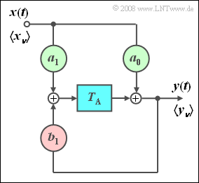
If at least one of the feedback coefficients is $b_{\mu} \ne 0$, then this is referred to as a recursive filter (see graphic on the right). The term IIR filter (Infinite Impulse Response) is also used for this, particularly in the English-language literature. This filter is dealt with in detail in the trial implementation.

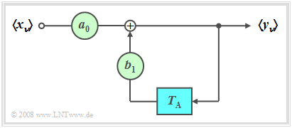
If all forward coefficients are also identical $a_\mu = 0$ with the exception of $a_0$, a purely recursive filter is available (see graphic on the left).

Purely recursive first order filter

In the following we restrict ourselves to the special case “purely recursive filter of the first order”. This filter has the following properties:

The output value $y_ν$ depends (indirectly) on an infinite number of input values:

$$y_\nu = \sum\limits_{\mu = 0}^\infty {a_0 \cdot {b_1} ^\mu \cdot x_{\nu - \mu } .}$$

This shows the following calculation:

$$y_\nu = a_0 \cdot x_\nu + b_1 \cdot y_{\nu - 1} = a_0 \cdot x_\nu + a_0 \cdot b_1 \cdot x_{\nu - 1} + {b_1} ^2 \cdot y_{\nu - 2} = a_0 \cdot x_\nu + a_0 \cdot b_1 \cdot x_{\nu - 1} + a_0 \cdot {b_1} ^2 \cdot x_{\nu - 2} + {b_1} ^3 \cdot y_{\nu - 3} = \text{...}. $$

By definition, the discrete-time impulse response is the same as the output sequence if there is a single "one" at $t =0$ at the input.

$$h(t)= \sum\limits_{\mu = 0}^\infty {a_0 \cdot {b_1} ^\mu \cdot \delta ( {t - \mu \cdot T_{\rm A} } )}\hspace{0.3cm} \Rightarrow \hspace{0.3cm}〈\hspace{0.05cm}h_\mu\hspace{0.05cm}〉= 〈\hspace{0.05cm}a_0, \ a_0\cdot {b_1}, \ a_0\cdot {b_1}^2 \ \text{...} \hspace{0.05cm}〉.$$

$\text{Conclusion:}$ With a recursive filter, the (discrete-time) impulse response extends to infinity with $M = 1$:

For reasons of stability, $b_1 < 1$ must apply.
With $b_1 = 1$ the impulse response $h(t)$ would extend to infinity and with $b_1 > 1$ the variable $h(t)$ would even continue to infinity.
With such a recursive filter of the first order, each individual Dirac delta line is exactly the factor $b_1$ smaller than the previous Dirac delta line:

$$h_{\mu} = h(\mu \cdot T_{\rm A}) = {b_1} \cdot h_{\mu -1}.$$

Discrete-time impulse response

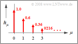
$\text{Example 3:}$ The graphic opposite shows the discrete-time impulse response $〈\hspace{0.05cm}h_\mu\hspace{0.05cm}〉$ of a recursive filter of the first order with the parameters $a_0 = 1$ and $b_1 = 0.6$.

The (discrete-time) course is exponentially falling and extends to infinity.
The ratio of the weights of two successive Dirac deltas is $b_1 = 0.6$.

Recursive filter as a sine generator

Proposed filter structure

The graphic shows a second-order digital filter that is suitable for generating a discrete-time sine function on a digital signal processor (DSP) if the input sequence $\left\langle \hspace{0.05cm} {x_\nu } \hspace{0.05cm}\right\rangle$ a (discrete-time) Dirac delta function is:

$$\left\langle \hspace{0.05cm}{y_\nu }\hspace{0.05cm} \right\rangle = \left\langle {\, \sin ( {\nu \cdot T_{\rm A} \cdot \omega _0 } )\, }\right\rangle .$$

The five filter coefficients result from the: "$Z$-transform":

$$Z \big \{ {\sin ( {\nu T{\rm A}\cdot \omega _0 } )} \big \} = \frac{{z \cdot \sin \left( {\omega _0 \cdot T_{\rm A}} \right)}}{{z^2 - 2 \cdot z \cdot \cos \left( {\omega _0 \cdot T_{\rm A}} \right) + 1}}.$$

After implementing this equation using a second-order recursive filter, the following filter coefficients are obtained:

$$a_0 = 0,\quad a_1 = \sin \left( {\omega _0 \cdot T_{\rm A}} \right),\quad a_2 = 0, \quad b_1 = 2 \cdot \cos \left( {\omega _0 \cdot T_{\rm A}} \right),\quad b_2 = - 1.$$

The filter coefficients $a_0$ and $a_2$ can be omitted and $b_2=-1$ has a fixed value.
The angular frequency $\omega_0$ of the sine wave is therefore only determined by $a_0$ and $a_0$.

$\text{Example 3:}$ Let $a_1 = 0.5$, $b_1 = \sqrt 3$, $x_0 = 1$ and $x_{\nu \hspace{0.05cm}\ne\hspace{0.05cm} 0} = 0$.

(1) Then the following applies to the initial values $y_\nu$ at times $\nu \ge 0$:

$y_0 = 0;$
$y_1 = 0.5$ ⇒ the "$1$" at the input only has an effect at time $\nu = 1$ because of $a_0= 0$ at the output;
$y_2 = b_1 \cdot y_1 - y_0 = {\sqrt 3 }/{2} \approx 0.866$ ⇒ with $\nu = 2$ the recursive part of the filter also takes effect;
$y_3 = \sqrt 3 \cdot y_2 - y_1 = \sqrt 3 \cdot {\sqrt 3 }/{2} - {1}/{2} = 1$ ⇒ for $\nu \ge 2$ the filter is purely recursive: $y_\nu = b_1 \cdot y_{\nu - 1} - y_{\nu - 2}$;
$y_4 = \sqrt 3 \cdot y_3 - y_2 = \sqrt 3 \cdot 1 - {\sqrt 3 }/{2} = {\sqrt 3 }/{2};$
$y_5 = \sqrt 3 \cdot y_4 - y_3 = \sqrt 3 \cdot {\sqrt 3 }/{2} - 1 = 0.5;$
$y_6 = \sqrt 3 \cdot y_5 - y_4 = \sqrt 3 \cdot {1}/{2} - {\sqrt 3 }/{2} = 0;$
$y_7 = \sqrt 3 \cdot y_6 - y_5 = \sqrt 3 \cdot 0 - {1}/{2} = - 0.5.$

(2) By continuing the recursive algorithm one gets for large $\nu$–values: $y_\nu = y_{\nu - 12}$ ⇒ $T_0/T_{\rm A}= 12.$

Exercises

First select the number 1 ... 10 of the task to be processed.
A task description is displayed. The parameter values are adjusted.
Solution after pressing "Sample Solution".
The number 0 corresponds to a "reset": Same setting as when the program was started.

(1) The filter coefficients are $a_0=0.25$, $a_1=0.5$, $a_2=0.25$, $b_1=b_2=0$. Which filter is it?
Interpret the impulse response $〈h_ν〉$, the step response $〈\sigma_ν〉$ and the rectangular response $〈\rho_ν^{(2, 8)}〉$, each in a discrete-time representation.

Due to the missing $b$ coefficients, it is a non-recursive digital filter ⇒ FIR filter (Finite Impulse Response).
The impulse response consists of $M+1=3$ Dirac delta lines according to the $a$ coefficients: $〈h_ν〉= 〈a_0, \ a_1,\ a_2〉= 〈0.25, \ 0.5,\ 0.25,\ 0, \ 0, \ 0,\text{...}〉 $.
The step response is: $〈\sigma_ν〉= 〈0.25, \ 0.75,\ 1,\ 1, \ 1, \ 1,\text{...}〉 $. The final value is equal to the DC signal transfer factor $H(f=0)=a_0+a_1+a_2 = 1$.
The distortions with rise and fall can also be seen from the rectangular response $〈\rho_ν^{(2, 8)}〉= 〈0,\ 0, 0.25, \ 0.75,\ 1,\ 1, \ 1, \ 1, \ 1, \ 0.75, \ 0.25, \ \text{...}〉$.

(2) How do the results differ with $a_2=-0.25$?

Taking into account $H(f=0)= 0.5$ there are comparable consequences ⇒ Step response: $〈\sigma_ν〉= 〈0.25, \ 0.75,\ 0.5,\ 0.5, \ 0.5, \ 0.5,\text{...}〉 $.

(3) Now let the filter coefficients $a_0=1$, $b_1=0.9$ and $a_1=a_2= b_2=0$. Which filter is it? Interpret the impulse response $〈h_ν〉$.

It is a recursive digital filter ⇒ IIR filter (Infinite Impulse Response) of the first order. It is the discrete-time analogon of the RC low-pass.
Starting from $h_0= 1$ is $h_1= h_0 \cdot b_0= 0.9$, $h_2= h_1 \cdot b_0= b_0^2=0.81$, $h_3= h_2 \cdot b_0= b_0^3=0.729$, and so on ⇒ $〈h_ν〉$ extends to infinity.
Impulse response $h(t) = {\rm e}^{-t/T}$ with $T$: intersection $($Tangente bei $t=0$, Abscissa$)$ ⇒ $h_\nu= h(\nu \cdot T_{\rm A}) = {\rm e}^{-\nu/(T/T_{\rm A})}$ with $T/T_{\rm A} = 1/(h_0-h_1)= 10$.
So: The values of the continuous time differ from the discrete-time impulse response. This results in the values $1.0, \ 0.9048,\ 0.8187$ ...

(4) The filter setting is retained. Interpret the step response $〈h_ν〉$ and the rectangular response $〈\rho_ν^{(2, 8)}〉$. What is the value for $H(f=0)$?

The step response is the integral over the impulse response: $\sigma(t) = T \cdot (1-{\rm e}^{-t/T}) ]$ ⇒ $\sigma_\nu= 10 \cdot (1-{\rm e}^{-\nu/10})$ ⇒ $\sigma_0=1$, $\sigma_1=1.9$, $\sigma_2=2.71$, ...
For large $\nu$ values, the (discrete-time) step response tends to the DC signal transmission factor $H(f=0)= 10$: $\sigma_{40}=9.867$, $\sigma_{50}=9.954$, $\sigma_\infty=10$.
The rectangular response $〈\rho_ν^{(2, 8)}〉$ increases with a delay of $2$ in the same way as $〈\sigma_ν〉$. In the area $\nu \ge 8$ the $\rho_ν$ values decrease exponentially.

(5) We continue to consider the filter with $a_0=1$, $b_1=0.9$, $a_1=a_2=b_2=0$. What is the output sequence $〈y_ν〉$ for the input sequence $〈x_ν〉= 〈1,\ 0,\ -0.5〉$?
Note: The task can also be solved with this program, although the constellation considered here cannot be set directly.

You can help yourself by setting the coefficient $a_2=-0.5$ and reducing the input sequence to $〈x_ν〉= 〈1,\ 0,\ 0,\ \text{ ...}〉$ ⇒ „Dirac delta function”.
The actual impulse response of this filter $($with $a_2=0)$ was determined in task (3): $h_0= 1$, $h_1= 0.9$, $h_2= 0.81$, $h_3= 0.729$, $h_4= 0.646$.
The solution to this problem is: $y_0 = h_0= 1$, $y_1= h_1= 0.9$, $y_2 =h_2-h_0/2= 0.31$, $y_3 =h_3-h_1/2= 0.279$, $y_4 =h_4-h_2/2= 0.251$.
Caution: Step response and rectangular response now refer to the fictitious filter $($with $a_2=-0.5)$ and not to the actual filter $($with $a_2=0)$.

(6) Consider and interpret the impulse response and the step response for the filter coefficients $a_0=1$, $b_1=1$, $a_1=a_2= b_2=0$.

The system is unstable: A discrete-time Dirac delta function at input $($at time $t=0)$ causes an infinite number of Dirac deltas of the same height in the output signal.
A discrete-time step function at the input causes an infinite number of Dirac deltas with monotonically increasing weights (to infinity) in the output signal.

(7) Consider and interpret the impulse response and step response for the filter coefficients $a_0=1$, $b_1=-1$, $a_1=a_2= b_2=0$.

In contrast to exercise (6), the weights of the impulse response $〈h_ν〉$ are not constantly equal to $1$, but alternating $\pm 1$. The system is unstable too.
With the jump response $〈\sigma_ν〉$, however, the weights alternate between $0$ $($with even $\nu)$ and $1$ $($with odd $\nu)$.

(8) We consider the "sine generator": $a_1=0.5$, $b_1=\sqrt{3}= 1.732$, $b_2=-1.$ Compare the impulse response with the calculated values in $\text{Example 4}$.
How do the parameters $a_1$ and $b_1$ influence the period duration $T_0/T_{\rm A}$ and the amplitude $A$ of the sine function?

$〈x_ν〉=〈1, 0, 0, \text{...}〉$ ⇒ $〈y_ν〉=〈0, 0.5, 0.866, 1, 0.866, 0.5, 0, -0.5, -0.866, -1, -0.866, -0.5, 0, \text{...}〉$ ⇒ sine, period $T_0/T_{\rm A}= 12$, amplitude $1$.
The increase/decrease of $b_1$ leads to the larger/smaller period $T_0/T_{\rm A}$ and the larger/smaller amplitude $A$. $b_1 < 2$ must apply.
$a_1$ only affects the amplitude, not the period. There is no value limit for $a_1$. If $a_1$ is negative, the minus sine function results.

(9) The basic setting is retained. Which $a_1$ and $b_1$ result in a sine function with period $T_0/T_{\rm A}=16$ and amplitude $A=1$?

Trying with $b_1= 1.8478$ actually achieves the period duration $T_0/T_{\rm A}=16$. However, this increases the amplitude to $A=1.307$.
Adjusting the parameter $a_1= 0.5/1.307=0.3826$ then leads to the desired amplitude $A=1$.
Or you can calculate this as in the example: $b_1 = 2 \cdot \cos ( {2{\rm{\pi }}\cdot{T_{\rm A}}/{T_0 }})= 2 \cdot \cos (\pi/8)=1.8478$, $a_1 = \sin (\pi/8)=0.3827$.

(10) We continue with the "sine generator". What modifications do you have to make to generate a "cosine"?

With $a_1=0.3826$, $b_1=1.8478$, $b_2=-1$ and $〈x_ν〉=〈1, 1, 1, \text{...}〉$ is the output sequence $〈y_ν〉$ the discrete-time analogon of the step response $\sigma(t)$.
The step response is the integral over $\sin(\pi\cdot\tau/8)$ within the limits of $\tau=0$ to $\tau=t$ ⇒ $\sigma(t)=-8/\pi\cdot\cos(\pi\cdot\tau/8)+1$.
If you change $a_1=0.3826$ on $a_1=-0.3826\cdot\pi/8=-0.1502$, then $\sigma(t)=\cos(\pi\cdot\tau/8)-1$ ⇒ Values between $0$ and $-2$.
Would you still in the block diagram $z_\nu=y_\nu+1$ add, then $z_\nu$ a discrete-time cosine curve with $T_0/T_{\rm A}=16$ and $A=1$.

Applet Manual

Screenshot Korrektur

(A) Auswahl der Quellensymbolfolge: $\rm A$, $\rm B$ oder $\rm C$

(B) Programmoptionen
$($Zufallsfolge, blockweise RDS-Berechnung, Gesamtansicht, Reset$)$

(C) "MS43" oder "MMS43"

(D) Berechnung der "Running Digital Sum"

(E) Blockweise Bitänderung

(F) Grafikbereich für das Quellensignal $q(t)$

(G) Grafikbereich für das Codersignal $c(t)$

(H) Gesamtdarstellung der Werte ${\it \Sigma}_0,\ {\it \Sigma}_1, \ {\it \Sigma}_2, \ {\it \Sigma}_4$ für "MS43" und "MMS43"

(I) Aufgabenauswahl

(I) Fragen und Lösungen

About the authors

This interactive calculation tool was designed and implemented at the chair for communications engineering at the Technische Universität München.

The first version was created in 2005 by Bettina Hirner as part of her diploma thesis with “FlashMX – Actionscript” (Supervisor: Günter Söder).
In 2020 the program was redesigned by André Schulz (Bachelor thesis LB, Supervisors: Benedikt Leible and Tasnád Kernetzky ) via "HTML5".

Once again: Open Applet in new Tab

Open Applet in a new tab