Exercise 1.16Z: Bounds for the Gaussian Error Function

• Return to book

Function  ${\rm Q}(x)$  and approximations;
it holds:  ${\rm Q_u}(x)\le{\rm Q}(x)\le{\rm Q_o}(x)$

The probability that a zero-mean Gaussian random variable  $n$  with standard deviation  $\sigma$   ⇒   variance  $\sigma^2$  is greater in magnitude than a given value  $A$  is equal to

$${\rm Pr}(n > A) = {\rm Pr}(n < -A) ={\rm Q}(A/\sigma) \hspace{0.05cm}.$$

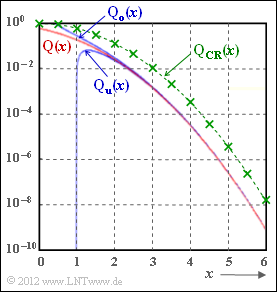
Here is used one of the most important functions for Communications Engineering  (drawn in red in the diagram):  
the  "complementary Gaussian error function"

$${\rm Q} (x) = \frac{\rm 1}{\sqrt{\rm 2\pi}}\int_{\it x}^{+\infty}\rm e^{\it -u^{\rm 2}/\rm 2}\,d \it u \hspace{0.05cm}.$$

${\rm Q}(x)$  is a monotonically decreasing function with  ${\rm Q}(0) = 0.5$.  For very large values of  $x$   ⇒   ${\rm Q}(x)$ tends $\to 0$.

The integral of the ${\rm Q}$–function is not analytically solvable and is usually given in tabular form.  From the literature,  however,  manageable approximations or bounds for positive  $x$  values are known:

• the  "upper bound"   ⇒   upper   $($German:  "obere"   ⇒   subscript: "o"$)$  blue curve in adjacent graph,  valid for  $x > 0$:

$${\rm Q_o}(x)=\frac{\rm 1}{\sqrt{\rm 2\pi}\cdot x}\cdot {\rm e}^{-x^{\rm 2}/\rm 2}\hspace{0.15cm} \ge \hspace{0.15cm} {\rm Q} (x) \hspace{0.05cm},$$

• the  "lower bound"   ⇒   upper   $($German:  "untere"   ⇒   subscript: "u"$)$  blue curve in adjacent graph,  valid for  $x > 1$:

$${\rm Q_u}(x)=\frac{\rm 1-{\rm 1}/{\it x^{\rm 2}}}{\sqrt{\rm 2\pi}\cdot x}\cdot \rm e^{-x^{\rm 2}/\rm 2} \hspace{0.15cm} \le \hspace{0.15cm} {\rm Q} (x) \hspace{0.05cm},$$

• the  "Chernoff-Rubin bound"  $($green curve in the graph, drawn for  $K = 1)$:

$${\rm Q_{CR}}(x)=K \cdot {\rm e}^{-x^{\rm 2}/\rm 2} \hspace{0.15cm} \ge \hspace{0.15cm} {\rm Q} (x) \hspace{0.05cm}.$$

In the exercise it is to be investigated to what extent these bounds can be used as approximations for  ${\rm Q}(x)$  and what corruptions result.

Hints:

• This exercise belongs to the chapter  "Bounds for block error probability".

• Reference is also made to the chapter  "Gaussian distributed random variables"  in the book  "Stochastic Signal Theory".

• The exercise provides some important hints for solving  "Exercise 1.16",  in which  ${\rm Q}_{\rm CR}(x)$  is used to derive the   "Bhattacharyya Bound"  for the AWGN channel.

• Further we refer to the interactive HTML5/JavaScript applet  "Complementary Gaussian error functions".

Questions

1

What values do the upper and lower bounds for  $x = 4$  provide?

${\rm Q_{o}}(x = 4) \ = \ $ $\ \cdot 10^{-5}$

${\rm Q_{u}}(x = 4) \ = \ $ $\ \cdot 10^{-5}$

2

What statements hold for the functions  ${\rm Q_{o}}(x)$  and  ${\rm Q_{u}}(x)$?

	For  $x ≥ 2$:  Both bounds are usable.
	For  $x < 1$:  ${\rm Q_{u}}(x)$  is unusable   $($because  ${\rm Q_{u}}(x)< 0)$.
	For  $x < 1$:  ${\rm Q_{o}}(x)$  is unusable  $($because  ${\rm Q_{o}}(x)> 1)$.

3

By what factor is the Chernoff-Rubin Bound above  ${\rm Q_{o}}(x)$?

${\rm Q}_{\rm CR}(x = 2)/{\rm Q_{o}}(x = 2 ) \ = \ $

${\rm Q}_{\rm CR}(x = 4)/{\rm Q_{o}}(x = 4 ) \ = \ $

${\rm Q}_{\rm CR}(x = 6)/{\rm Q_{o}}(x = 6 ) \ = \ $

4

Determine  $K$  such that  $K \cdot {\rm Q}_{\rm CR}(x)$  is as close as possible to  ${\rm Q}(x)$  and at the same time  ${\rm Q}(x) ≤ K · {\rm Q}_{\rm CR}(x)$  is observed for all  $x > 0$ .

$K \ = \ $

Solution

Solution

(1)  The upper bound is:

$${\rm Q_o}(x)=\frac{1}{\sqrt{\rm 2\pi}\cdot x}\cdot {\rm e}^{-x^{\rm 2}/\rm 2} \hspace{0.3cm} \Rightarrow \hspace{0.3cm} {\rm Q_o}(4 )=\frac{1}{\sqrt{\rm 2\pi}\cdot 4}\cdot {\rm e}^{-8 }\hspace{0.15cm}\underline{\approx 3.346 \cdot 10^{-5}}\hspace{0.05cm}.$$

• The lower bound can be converted as follows:

$${\rm Q_u}( x)=(1-1/x^2) \cdot {\rm Q_o}(x) \hspace{0.3cm} \Rightarrow \hspace{0.3cm} {\rm Q_u}(4 ) \hspace{0.15cm}\underline{\approx 3.137 \cdot 10^{-5}} \hspace{0.05cm}.$$

• The relative deviations from the  actual  value  ${\rm Q}(4) = 3.167 · 10^{–5}$  are  $+5\%$  resp.  $–1\%$.

(2)  Correct are the  solutions 1 and 2:

• For  $x = 2$,  the actual function value  ${\rm Q}(x) = 2.275 \cdot 10^{-2}$  is bounded by  ${\rm Q_{o}}(x) = 2.7 \cdot 10^{-2}$  and  ${\rm Q_u}(x) = 2.025 \cdot 10^{-2}$, respectively.

• The relative deviations are therefore  $18.7\%$ resp.  $-11\%,$.

• The last statement is wrong:   Only for  $x < 0.37$   ⇒   ${\rm Q_o}(x) > 1$  is valid.

(3)  For the quotient of  ${\rm Q}_{\rm CR}(x)$  and  ${\rm Q_o}(x)$,  according to the given equations:

$$q(x) = \frac{{\rm Q_{CR}}(x)}{{\rm Q_{o}}(x)} = \frac{{\rm exp}(-x^2/2)}{{\rm exp}(-x^2/2)/({\sqrt{2\pi} \cdot x})} = {\sqrt{2\pi} \cdot x}$$

$$\Rightarrow \hspace{0.3cm} q(x) \approx 2.5 \cdot x \hspace{0.3cm} \Rightarrow \hspace{0.3cm} q(x =2) \hspace{0.15cm}\underline{=5}\hspace{0.05cm}, \hspace{0.2cm}q(x =4)\hspace{0.15cm}\underline{=10}\hspace{0.05cm}, \hspace{0.2cm}q(x =6) \hspace{0.15cm}\underline{=15}\hspace{0.05cm}.$$

• The larger the abscissa value  $x$  is,  the more inaccurately  ${\rm Q}(x)$  is approximated by  ${\rm Q}_{\rm CR}(x)$.

• When looking at the graph in the information section,  I first had the impression that  ${\rm Q}_{\rm CR}(x)$  results from  ${\rm Q}(x)$  by shifting to the right or shifting up. 

• But this is only an optical illusion and does not correspond to the facts.

(4)  With  $\underline{K = 0.5}$  the new bound  $0.5 \cdot {\rm Q}_{\rm CR}(x)$  for  $x = 0$  agrees exactly with ${\rm Q}(x=0) = 0.500$.

• For larger abscissa values,  the falsification  $q \approx 1.25 \cdot x$  thus also becomes only half as large.