Exercise 3.3: Code Sequence Calculation via U(D) and G(D)

Considered generator matrix

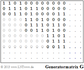
The upper left section of the generator matrix $\mathbf{G}$ is shown for the considered convolutional code.

From this the partial matrices $\mathbf{G}_l$ are to be extracted under the boundary condition $m ≤ 2$ , with which then the transfer function matrix can be composed according to the following equation:

${\boldsymbol{\rm G}}(D) = \sum_{l = 0}^{m} {\boldsymbol{\rm G}}_l \cdot D\hspace{0.03cm}^l = {\boldsymbol{\rm G}}_0 + {\boldsymbol{\rm G}}_1 \cdot D + \ \text{...} \ \hspace{0.05cm}+ {\boldsymbol{\rm G}}_m \cdot D\hspace{0.03cm}^m \hspace{0.02cm}.$

Searched are the $n$ code sequences $\underline{x}^{(1)}, \ \underline{x}^{(2)}, \hspace{0.05cm} \text{...} \hspace{0.05cm} , \ \underline{x}^{(n)}$ , assuming the following information sequence:

$\underline{u} = (0\hspace{0.05cm},\hspace{0.05cm} 1\hspace{0.05cm},\hspace{0.05cm} 1\hspace{0.05cm},\hspace{0.05cm} 1\hspace{0.05cm},\hspace{0.05cm} 1\hspace{0.05cm},\hspace{0.05cm}0\hspace{0.05cm},\hspace{0.05cm} 1\hspace{0.05cm},\hspace{0.05cm} 0\hspace{0.05cm},\hspace{0.05cm} 1\hspace{0.05cm},\hspace{0.05cm} \text{...} \hspace{0.05cm}\hspace{0.05cm})$

This sequence is thereby divided into $k$ subsequences $\underline{u}^{(1)}, \ \underline{u}^{(2)}, \hspace{0.05cm} \text{...} \hspace{0.05cm} , \ \underline{u}^{(k)}$ to split.

From their D–transforms

${U}^{(1)}(D) \hspace{0.15cm}\bullet\!\!-\!\!\!-^{\hspace{-0.25cm}D}\!\!\!-\!\!\circ\hspace{0.15cm} \underline{u}^{(1)},\hspace{0.25cm} ...\hspace{0.25cm},\hspace{0.05cm} {U}^{(k)}(D) \hspace{0.15cm}\bullet\!\!-\!\!\!-^{\hspace{-0.25cm}D}\!\!\!-\!\!\circ\hspace{0.15cm} \underline{u}^{(k)}$

the vector

$\underline{U}(D) = (U^{(1)}(D), \hspace{0.05cm} \text{...} \hspace{0.05cm} , \ U^{(k)}(D))$ is formed.

Then applies to the code sequence vector in D–representation:

$\underline{X}(D) = \left (\hspace{0.05cm} {X}^{(1)}(D)\hspace{0.05cm}, \hspace{0.05cm} \text{...} \hspace{0.05cm}, \hspace{0.05cm} {X}^{(k)}(D)\hspace{0.05cm}\right ) = \underline{U}(D) \cdot {\boldsymbol{\rm G}}(D)\hspace{0.05cm}.$

Hints:

This exercise belongs to the chapter "Algebraic and Polynomial Description".

The underlying encoder here is identical to that of $\text{Exercise 3.2}$ .

Since also $\underline{u}$ remains the same code sequence $\underline{x}$ must result here as in Exercise 3.2. However, the solution paths of both exercises are fundamentally different.

Questions

Solution

(1) The generator matrix of a convolutional code has the general form:

${ \boldsymbol{\rm G}}=\begin{pmatrix} { \boldsymbol{\rm G}}_0 & { \boldsymbol{\rm G}}_1 & { \boldsymbol{\rm G}}_2 & \cdots & { \boldsymbol{\rm G}}_m & & & \\ & { \boldsymbol{\rm G}}_0 & { \boldsymbol{\rm G}}_1 & { \boldsymbol{\rm G}}_2 & \cdots & { \boldsymbol{\rm G}}_m & &\\ & & { \boldsymbol{\rm G}}_0 & { \boldsymbol{\rm G}}_1 & { \boldsymbol{\rm G}}_2 & \cdots & { \boldsymbol{\rm G}}_m &\\ & & & \ddots & \ddots & & & \ddots \end{pmatrix}\hspace{0.05cm}.$

From the graph on the information page, the $k × n$ partial matrices can be determined:

${ \boldsymbol{\rm G}}_0=\begin{pmatrix} 1 & 1 & 0 & 1 \\ 0 & 1 & 1 & 1 \\ 0 & 0 & 1 & 1 \end{pmatrix}\hspace{0.05cm},\hspace{0.2cm} { \boldsymbol{\rm G}}_1=\begin{pmatrix} 0 & 0 & 0 & 0 \\ 0 & 1 & 1 & 0 \\ 0 & 1 & 0 & 0 \end{pmatrix}\hspace{0.05cm},\hspace{0.2cm} { \boldsymbol{\rm G}}_2=\begin{pmatrix} 0 & 0 & 0 & 0 \\ 0 & 0 & 0 & 0 \\ 0 & 0 & 1 & 1 \end{pmatrix}\hspace{0.05cm}.$

The code parameters are thus: $\underline{n = 4}$ , $\underline{k = 3}$ , $\underline{m = 2}$ .

Hints:

The represented part of $\mathbf{G}$ would have the same appearance for $m > 2$ as for $m = 2$ .
This is why the additional specification $m ≤ 2$ was necessary.

(2) All proposed solutions are correct. According to the specification sheet

${\boldsymbol{\rm G}}(D) = {\boldsymbol{\rm G}}_0 + {\boldsymbol{\rm G}}_1 \cdot D + {\boldsymbol{\rm G}}_2 \cdot D^2 = \begin{pmatrix} 1 & 1 & 0 & 1 \\ 0 & 1+D & 1+D & 1 \\ 0 & D & 1+D^2 & 1+D^2 \end{pmatrix}\hspace{0.05cm}.$

(3) After splitting the information sequence

$\underline{u} = (0\hspace{0.05cm},\hspace{0.05cm} 1\hspace{0.05cm},\hspace{0.05cm} 1\hspace{0.05cm},\hspace{0.05cm} 1\hspace{0.05cm},\hspace{0.05cm} 1\hspace{0.05cm},\hspace{0.05cm}0\hspace{0.05cm},\hspace{0.05cm} 1\hspace{0.05cm},\hspace{0.05cm} 0\hspace{0.05cm},\hspace{0.05cm} 1\hspace{0.05cm}, ... \hspace{0.05cm})$

into the three partial sequences $\underline{u}^{(1)}$ , $\underline{u}^{(2)}$ , $\underline{u}^{(3)}$ and subsequent D–transformation we get:

$\underline{u}^{(1)} \hspace{-0.15cm} \ = \ \hspace{-0.15cm} (\hspace{0.05cm}0\hspace{0.05cm},\hspace{0.05cm}1\hspace{0.05cm},\hspace{0.05cm} 1\hspace{0.05cm}) \quad \circ\!\!-\!\!\!-^{\hspace{-0.25cm}D}\!\!\!-\!\!\bullet\quad {U}^{(1)}(D) = D + D^2 \hspace{0.05cm},$

$\underline{u}^{(2)} \hspace{-0.15cm} \ = \ \hspace{-0.15cm} (\hspace{0.05cm}1\hspace{0.05cm},\hspace{0.05cm}1\hspace{0.05cm},\hspace{0.05cm} 0\hspace{0.05cm}) \quad \circ\!\!-\!\!\!-^{\hspace{-0.25cm}D}\!\!\!-\!\!\bullet\quad {U}^{(2)}(D) = 1+D \hspace{0.05cm},$

$\underline{u}^{(3)} \hspace{-0.15cm} \ = \ \hspace{-0.15cm} (\hspace{0.05cm}1\hspace{0.05cm},\hspace{0.05cm}0\hspace{0.05cm},\hspace{0.05cm} 1\hspace{0.05cm}) \quad \circ\!\!-\!\!\!-^{\hspace{-0.25cm}D}\!\!\!-\!\!\bullet\quad {U}^{(3)}(D) = 1 + D^2 \hspace{0.05cm}.$

Accordingly, only the proposed solution 2 is correct.

(4) In the first column of $\mathbf{G}(D)$ there is only one " $1$ " in row 1, the other two matrix elements are zero.

This is a systematic code ⇒ $\underline{x}^{(1)} = \underline{u}^{(1)} = (0, \, 1, \, 1)$ .

Correct is the proposed solution 1.

(5) The D–transform $X^{(2)}(D)$ is obtained as the vector product

of the D–transform of the information sequence ⇒ $\underline{U}(D) = (U^{(1)}(D), \, U^{(2)}(D), \, U^{(3)}(D))$

and the second column of $\mathbf{G}(D)$ :

$X^{(2)}(D) \hspace{-0.15cm} \ = \ \hspace{-0.15cm} ( D + D^2) \cdot 1 + ( 1+D) \cdot ( 1+D) +( 1+D^2) \cdot D\hspace{0.03cm}=D + D^2 +1 +D +D + D^2 +D + D^3 = 1+D^3 \hspace{0.05cm}.$

Correct is the proposed solution 2: $\underline{x}^{(2)} = (1, \, 0, \, 0)$ . Since we are only interested in the first three bits, the contribution $D^3$ is not relevant.

(6) Analogous to subtask (5), we obtain here:

$X^{(3)}(D) \hspace{-0.15cm} \ = \ \hspace{-0.15cm} ( D + D^2) \cdot 0 + ( 1+D) \cdot ( 1+D) +( 1+D^2) \cdot ( 1+D^2)=1 + D + D + D^2 +1 + D^2 + D^2 + D^4 = D^2 + D^4 \hspace{0.05cm}.$

This gives $\underline{x}^{(3)} = (0, \, 0, \, 1)$ ⇒ Proposed solution 3.

The same result is obtained for $\underline{x}^{(4)}$ .

After joining all $n = 4$ subsequences, one obtains (of course) the same result as in $\text{Exercise 3.2}$ :

$\underline{x} = (0\hspace{0.05cm},\hspace{0.05cm} 1\hspace{0.05cm},\hspace{0.05cm} 0\hspace{0.05cm},\hspace{0.05cm} 0\hspace{0.05cm},\hspace{0.05cm} 1\hspace{0.05cm},\hspace{0.05cm}0\hspace{0.05cm},\hspace{0.05cm} 0\hspace{0.05cm},\hspace{0.05cm} 0\hspace{0.05cm},\hspace{0.05cm} 1\hspace{0.05cm}, \hspace{0.05cm} 0\hspace{0.05cm},\hspace{0.05cm} 1\hspace{0.05cm},\hspace{0.05cm} 1\hspace{0.05cm},\hspace{0.05cm}\text{ ...} \hspace{0.05cm})\hspace{0.05cm}.$

	The $\mathbf{G}(D)$ element in row 1, column 1 is " $1$ ".
	The $\mathbf{G}(D)$ element in row 2, column 2 is " $1 + D$ ".
	The $\mathbf{G}(D)$ element in row 3, column 3 is " $1 + D^2$ ".

	$U^{(1)}(D) = 1$ ,
	$U^{(2)}(D) = 1 + D$ ,
	$U^{(3)}(D) = D^2$ .

	$\underline{x}^{(1)} = (0, \, 1, \, 1, \, \hspace{0.05cm} \text{...} \hspace{0.05cm})$ ,
	$\underline{x}^{(1)} = (1, \, 0, \, 0, \, \hspace{0.05cm} \text{...} \hspace{0.05cm})$ ,
	$\underline{x}^{(1)} = (0, \, 0, \, 1, \, \hspace{0.05cm} \text{...} \hspace{0.05cm})$ .

	$\underline{x}^{(2)} = (0, \, 1, \, 1, \, \hspace{0.05cm} \text{...} \hspace{0.05cm})$ ,
	$\underline{x}^{(2)} = (1, \, 0, \, 0, \, \hspace{0.05cm} \text{...} \hspace{0.05cm})$ ,
	$\underline{x}^{(2)} = (0, \, 0, \, 1, \, \hspace{0.05cm} \text{...} \hspace{0.05cm})$ .

	$\underline{x}^{(3)} = (0, \, 1, \, 1, \, \hspace{0.05cm} \text{...} \hspace{0.05cm})$ ,
	$\underline{x}^{(3)} = (1, \, 0, \, 0, \, \hspace{0.05cm} \text{...} \hspace{0.05cm})$ ,
	$\underline{x}^{(3)} = (0, \, 0, \, 1, \, \hspace{0.05cm} \text{...} \hspace{0.05cm})$ .