Exercise 4.15: PDF and Covariance Matrix
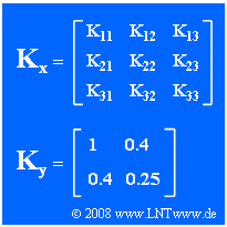
We consider here the three-dimensional random variable $\mathbf{x}$, whose commonly represented covariance matrix $\mathbf{K}_{\mathbf{x}}$ is given in the upper graph. The random variable has the following properties:
- The three components are Gaussian distributed and it holds for the elements of the covariance matrix:
- $$K_{ij} = \sigma_i \cdot \sigma_j \cdot \rho_{ij}.$$
- Let the elements on the main diagonal be known:
- $$ K_{11} =1, \ K_{22} =0, \ K_{33} =0.25.$$
- The correlation coefficient between the coefficients $x_1$ and $x_3$ is $\rho_{13} = 0.8$.
In the second part of the exercise, consider the random variable $\mathbf{y}$ with the two components $y_1$ and $y_2$ whose covariance matrix $\mathbf{K}_{\mathbf{y}}$ is determined by the given numerical values $(1, \ 0.4, \ 0.25)$ .
The probability density function $\rm (PDF)$ of a zero mean Gaussian two-dimensional random variable $\mathbf{y}$ is as specified on page "Relationship between covariance matrix and PDF" with $N = 2$:
- $$\mathbf{f_y}(\mathbf{y}) = \frac{1}{{2 \pi \cdot \sqrt{|\mathbf{K_y}|}}}\cdot {\rm e}^{-{1}/{2} \hspace{0.05cm}\cdot\hspace{0.05cm} \mathbf{y} ^{\rm T}\hspace{0.05cm}\cdot\hspace{0.05cm}\mathbf{K_y}^{-1} \hspace{0.05cm}\cdot\hspace{0.05cm} \mathbf{y} }= C \cdot {\rm e}^{-\gamma_1 \hspace{0.05cm}\cdot\hspace{0.05cm} y_1^2 \hspace{0.1cm}+\hspace{0.1cm} \gamma_2 \hspace{0.05cm}\cdot\hspace{0.05cm} y_2^2 \hspace{0.1cm}+\hspace{0.1cm}\gamma_{12} \hspace{0.05cm}\cdot\hspace{0.05cm} y_1 \hspace{0.05cm}\cdot\hspace{0.05cm} y_2 }.$$
- In the subtasks (5) and (6) the prefactor $C$ and the further PDF coefficients $\gamma_1$, $\gamma_2$ and $\gamma_{12}$ are to be calculated according to this vector representation.
- In contrast, the corresponding equation in conventional approach according to the chapter "Two-dimensional Gaussian Random Variables" would be:
- $$f_{y_1,\hspace{0.1cm}y_2}(y_1,y_2)=\frac{\rm 1}{\rm 2\pi \sigma_1 \sigma_2 \sqrt{\rm 1-\rho^2}}\cdot\exp\Bigg[-\frac{\rm 1}{\rm 2 (1-\rho^{\rm 2})}\cdot(\frac { y_1^{\rm 2}}{\sigma_1^{\rm 2}}+\frac { y_2^{\rm 2}}{\sigma_2^{\rm 2}}-\rm 2\rho \frac{{\it y}_1{\it y}_2}{\sigma_1 \cdot \sigma_2}) \rm \Bigg].$$
Hints:
- The exercise belongs to the chapter Generalization to N-Dimensional Random Variables.
- Some basics on the application of vectors and matrices can be found in the sections "Determinant of a Matrix" and Inverse of a Matrix .
- Reference is also made to the chapter "Two-Dimensional Gaussian Random Variables".
Questions
Solution
- On the basis of the covariance matrix $\mathbf{K}_{\mathbf{x}}$ it is not possible to make any statement about whether the underlying random variable $\mathbf{x}$ is zero mean or mean-invariant, since any mean value $\mathbf{m}$ is factored out.
- To make statements about the mean, the correlation matrix $\mathbf{R}_{\mathbf{x}}$ would have to be known.
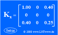
- From $K_{22} = \sigma_2^2 = 0$ it follows necessarily that all other elements in the second row $(K_{21}, K_{23})$ and the second column $(K_{12}, K_{32})$ are also zero.
- On the other hand, the third statement is false: The elements are symmetric about the main diagonal, so that always $K_{31} = K_{13}$ must hold.
(2) From $K_{11} = 1$ and $K_{33} = 0.25$ follow directly $\sigma_1 = 1$ and $\sigma_3 = 0.5$.
- Taken together with the correlation coefficient $\rho_{13} = 0.8$ (see specification sheet), we thus obtain:
- $$K_{13} = K_{31} = \sigma_1 \cdot \sigma_2 \cdot \rho_{13}\hspace{0.15cm}\underline{= 0.4}.$$
(3) The determinant of the matrix $\mathbf{K_y}$ is:
- $$|{\mathbf{K_y}}| = 1 \cdot 0.25 - 0.4 \cdot 0.4 \hspace{0.15cm}\underline{= 0.09}.$$
(4) According to the statements on the pages "Determinant of a Matrix" and "Inverse of a Matrix" holds:
- $${\mathbf{I_y}} = {\mathbf{K_y}}^{-1} = \frac{1}{|{\mathbf{K_y}}|}\cdot \left[ \begin{array}{cc} 0.25 & -0.4 \\ -0.4 & 1 \end{array} \right].$$
- With $|\mathbf{K_y}|= 0.09$ therefore holds further:
- $$I_{11} = {25}/{9}\hspace{0.15cm}\underline{ = 2.777};\hspace{0.3cm} I_{12} = I_{21} = -40/9 \hspace{0.15cm}\underline{ = -4.447};\hspace{0.3cm}I_{22} = {100}/{9} \hspace{0.15cm}\underline{= 11.111}.$$
(5) A comparison of $\mathbf{K_y}$ and $\mathbf{K_x}$ with constraint $K_{22} = 0$ shows that $\mathbf{x}$ and $\mathbf{y}$ are identical random variables if one sets $y_1 = x_1$ and $y_2 = x_3$ .
- Thus, for the PDF parameters:
- $$\sigma_1 =1, \hspace{0.3cm} \sigma_2 =0.5, \hspace{0.3cm} \rho =0.8.$$
- The prefactor according to the general PDF definition is thus:
- $$C =\frac{\rm 1}{\rm 2\pi \cdot \sigma_1 \cdot \sigma_2 \cdot \sqrt{\rm 1-\rho^2}}= \frac{\rm 1}{\rm 2\pi \cdot 1 \cdot 0.5 \cdot 0.6}= \frac{1}{0.6 \cdot \pi} \hspace{0.15cm}\underline{\approx 0.531}.$$
- With the determinant calculated in subtask (3) we get the same result:
- $$C =\frac{\rm 1}{\rm 2\pi \sqrt{|{\mathbf{K_y}}|}}= \frac{\rm 1}{\rm 2\pi \sqrt{0.09}} = \frac{1}{0.6 \cdot \pi}.$$
(6) The inverse matrix computed in subtask (4) can also be written as follows:
- $${\mathbf{I_y}} = \frac{5}{9}\cdot \left[ \begin{array}{cc} 5 & -8 \\ -8 & 20 \end{array} \right].$$
- So the argument $A$ of the exponential function is:
- $$A = \frac{5}{18}\cdot{\mathbf{y}}^{\rm T}\cdot \left[ \begin{array}{cc} 5 & -8 \\ -8 & 20 \end{array} \right]\cdot{\mathbf{y}} =\frac{5}{18}\left( 5 \cdot y_1^2 + 20 \cdot y_2^2 -16 \cdot y_1 \cdot y_2\right).$$
- By comparing coefficients, we get:
- $$\gamma_1 = \frac{25}{18} \approx 1.389; \hspace{0.3cm} \gamma_2 = \frac{100}{18} \approx 5.556; \hspace{0.3cm} \gamma_{12} = - \frac{80}{18} \approx -4,444.$$
- According to the conventional procedure, the same numerical values result:
- $$\gamma_1 =\frac{\rm 1}{\rm 2\cdot \sigma_1^2 \cdot ({\rm 1-\rho^2})}= \frac{\rm 1}{\rm 2 \cdot 1 \cdot 0.36} \hspace{0.15cm}\underline{ \approx 1.389},$$
- $$\gamma_2 =\frac{\rm 1}{\rm 2 \cdot\sigma_2^2 \cdot ({\rm 1-\rho^2})}= \frac{\rm 1}{\rm 2 \cdot 0.25 \cdot 0.36} = 4 \cdot \gamma_1 \hspace{0.15cm}\underline{\approx 5.556},$$
- $$\gamma_{12} =-\frac{\rho}{ \sigma_1 \cdot \sigma_2 \cdot ({\rm 1-\rho^2})}= -\frac{\rm 0.8}{\rm 1 \cdot 0.5 \cdot 0.36} \hspace{0.15cm}\underline{ \approx -4.444}.$$

