Statistical Dependence and Independence

General definition of statistical dependence

So far we have not paid much attention to »statistical dependence« between events, even though we have already used it as in the case of two »disjoint sets«:

If an element belongs to $A$ ,

it cannot with certainty also be contained in the disjoint set $B$ .

The strongest form of dependence at all is such a »deterministic dependence« between two sets or two events. Less pronounced is the statistical dependence. Let us start with its complement:

$\text{Definitions:}$

$(1)$ Two events $A$ and $B$ are called »statistically independent«, if the probability of the intersection $A ∩ B$ is equal to the product of the individual probabilities:

${\rm Pr}(A \cap B) = {\rm Pr}(A)\cdot {\rm Pr}(B).$

$(2)$ If this condition is not satisfied, then the events $A$ and $B$ are »statistically dependent«:

${\rm Pr}(A \cap B) \ne {\rm Pr}(A)\cdot {\rm Pr}(B).$

In some applications, statistical independence is obvious, for example, in the »coin toss« experiment. The probability for »heads« or »tails« is independent of whether »heads« or »tails« occurred in the last toss.

And also the individual results in the random experiment »throwing a roulette ball« are always statistically independent of each other under fair conditions, even if individual system players do not want to admit this.

In other applications, on the other hand, the question whether two events are statistically independent or not is not or only very difficult to answer instinctively. Here one can only arrive at the correct answer by checking the formal independence criterion given above, as the following example will show.

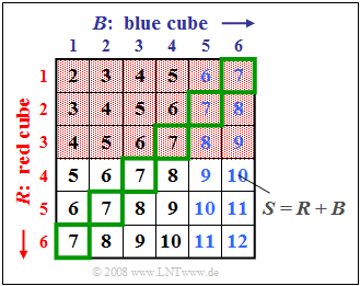
$\text{Example 1:}$ We consider the experiment »throwing two dice«, where the two dice $($ in graphic: "cubes" $)$ can be distinguished by their colors red $(R)$ and blue $(B)$ . The graph illustrates this fact, where the sum $S = R + B$ is entered in the two-dimensional field $(R, B)$ .

For the following description we define the following events:

Examples for statistically independent events

$A_1$ : The outcome of the red cube is $R < 4$ $($ red background $)$ ⇒ ${\rm Pr}(A_1) = 1/2$ ,
$A_2$ : The outcome of the blue cube is $B > 4$ $($ blue font $)$ ⇒ ${\rm Pr}(A_2) = 1/3$ ,
$A_3$ : The sum of the two cubes is $S = 7$ $($ green outline $)$ ⇒ ${\rm Pr}(A_3) = 1/6$ ,
$A_4$ : The sum of the two cubes is $S = 8$ ⇒ ${\rm Pr}(A_4) = 5/36$ ,
$A_5$ : The sum of the two cubes is $S = 10$ ⇒ ${\rm Pr}(A_5) = 3/36$ .

The graph can be interpreted as follows:

The two events $A_1$ and $A_2$ are statistically independent because the probability ${\rm Pr}(A_1 ∩ A_2) = 1/6$ of the intersection is equal to the product of the two individual probabilities ${\rm Pr}(A_1) = 1/2$ and ${\rm Pr}(A_2) = 1/3$ . Given the problem definition, any other result would also have been very surprising.

But also the events $A_1$ and $A_3$ are statistically independent because of ${\rm Pr}(A_1) = 1/2$ , ${\rm Pr}(A_3) = 1/6$ and ${\rm Pr}(A_1 ∩ A_3) = 1/12$ . The probability of intersection $(1/12)$ arises because three of the $36$ squares are both highlighted in red and outlined in green.

In contrast, there are statistical bindings between $A_1$ and $A_4$ because the probability of intersection ⇒ ${\rm Pr}(A_1 ∩ A_4) = 1/18 = 4/72$ is not equal to the product ${\rm Pr}(A_1) \cdot {\rm Pr}(A_4)= 1/2 \cdot 5/36 = 5/72$ .

The two events $A_1$ and $A_5$ are even disjoint ⇒ ${\rm Pr}(A_1 ∩ A_5) = 0$ : none of the boxes with red background is labeled $S=10$ .

This example shows that disjunctivity is a particularly pronounced form of statistical dependence.

Conditional probability

If there are statistical bindings between the two events $A$ and $B$ , the $($ unconditional $)$ probabilities ${\rm Pr}(A)$ and ${\rm Pr}(B)$ do not describe the situation unambiguously in the statistical sense. So-called »conditional probabilities« are then required.

$\text{Definitions:}$

$(1)$ The »conditional probability« of $A$ under condition $B$ can be calculated as follows:

${\rm Pr}(A\hspace{0.05cm} \vert \hspace{0.05cm} B) = \frac{ {\rm Pr}(A \cap B)}{ {\rm Pr}(B)}.$

$(2)$ Similarly, the conditional probability of $B$ under condition $A$ is:

${\rm Pr}(B\hspace{0.05cm} \vert \hspace{0.05cm}A) = \frac{ {\rm Pr}(A \cap B)}{ {\rm Pr}(A)}.$

$(3)$ Combining these two equations, we get $\text{Bayes'}$ theorem:

${\rm Pr}(B \hspace{0.05cm} \vert \hspace{0.05cm} A) = \frac{ {\rm Pr}(A\hspace{0.05cm} \vert \hspace{0.05cm} B)\cdot {\rm Pr}(B)}{ {\rm Pr}(A)}.$

Below are some properties of conditional probabilities:

Also a conditional probability lies always between $0$ and $1$ including these two limits: $0 \le {\rm Pr}(A \hspace{0.05cm} | \hspace{0.05cm} B) \le 1$ .
With constant condition $B$ , all calculation rules given in the chapter »Set Theory Basics« for the unconditional probabilities ${\rm Pr}(A)$ and ${\rm Pr}(B)$ still apply.
If the existing events $A$ and $B$ are disjoint, then ${\rm Pr}(A\hspace{0.05cm} | \hspace{0.05cm} B) = {\rm Pr}(B\hspace{0.05cm} | \hspace{0.05cm}A)= 0$ $($ agreement: event $A$ »exists« if ${\rm Pr}(A) > 0)$ .
If $B$ is a proper or improper subset of $A$ , then ${\rm Pr}(A \hspace{0.05cm} | \hspace{0.05cm} B) =1$ .
If two events $A$ and $B$ are statistically independent, their conditional probabilities are equal to the unconditional ones, as the following calculation shows:

${\rm Pr}(A \hspace{0.05cm} | \hspace{0.05cm} B) = \frac{{\rm Pr}(A \cap B)}{{\rm Pr}(B)} = \frac{{\rm Pr} ( A) \cdot {\rm Pr} ( B)} { {\rm Pr}(B)} = {\rm Pr} ( A).$

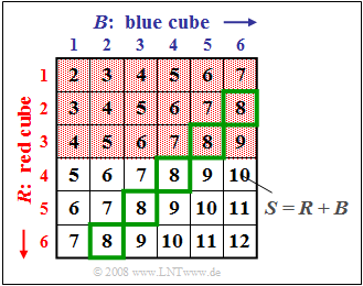
$\text{Example 2:}$ We again consider the experiment »Throwing two dice«, where $S = R + B$ denotes the sum of the red and blue dice $($ cube $)$ .

Example of statistically dependent events

Here we consider bindings between the two events

$A_1$ : »The outcome of the red cube is $R < 4$ « $($ red background $)$ ⇒ ${\rm Pr}(A_1) = 1/2$ ,

$A_4$ : »The sum of the two cubes is $S = 8$ « $($ green outline $)$ ⇒ ${\rm Pr}(A_4) = 5/36$ ,

and refer again to the event of $\text{Example 1}$ :

$A_3$ : »The sum of the two cubes is $S = 7$ « ⇒ ${\rm Pr}(A_3) = 1/6$ .

Regarding this graph, note:

There are statistical bindings between the both events $A_1$ and $A_4$ , since the probability of intersection ⇒ ${\rm Pr}(A_1 ∩ A_4) = 2/36 = 4/72$ is not equal to the product ${\rm Pr}(A_1) \cdot {\rm Pr}(A_4)= 1/2 \cdot 5/36 = 5/72$ .

The conditional probability ${\rm Pr}(A_1 \hspace{0.05cm} \vert \hspace{0.05cm} A_4) = 2/5$ can be calculated from the quotient of the »joint probability« ${\rm Pr}(A_1 ∩ A_4) = 2/36$ and the absolute probability ${\rm Pr}(A_4) = 5/36$ .

Since the events $A_1$ and $A_4$ are statistically dependent, the conditional probability ${\rm Pr}(A_1 \hspace{0.05cm}\vert \hspace{0.05cm} A_4) = 2/5$ $($ two of the five squares outlined in green are highlighted in red $)$ is not equal to the absolute probability ${\rm Pr}(A_1) = 1/2$ $($ half of all squares are highlighted in red $)$ .

Similarly, the conditional probability ${\rm Pr}(A_4 \hspace{0.05cm} \vert \hspace{0.05cm} A_1) = 2/18 = 1/9$ $($ two of the $18$ fields with a red background are outlined in green $)$ is unequal to the absolute probability ${\rm Pr}(A_4) = 5/36$ $($ a total of five of the $36$ fields are outlined in green $)$ .

This last result can also be derived using »Bayes' theorem«, for example:

${\rm Pr}(A_4 \hspace{0.05cm} \vert\hspace{0.05cm} A_1) = \frac{ {\rm Pr}(A_1 \hspace{0.05cm} \vert\hspace{0.05cm} A_4)\cdot {\rm Pr} ( A_4)} { {\rm Pr}(A_1)} = \frac{2/5 \cdot 5/36}{1/2} = 1/9.$

In contrast, the following conditional probabilities hold for $A_1$ and the statistically independent event $A_3$ , see $\text{Example 1}$ :

${\rm Pr}(A_{\rm 1} \hspace{0.05cm}\vert \hspace{0.05cm} A_{\rm 3}) = {\rm Pr}(A_{\rm 1}) = \rm 1/2\hspace{0.5cm}{\rm resp.}\hspace{0.5cm}{\rm Pr}(A_{\rm 3} \hspace{0.05cm} \vert \hspace{0.05cm} A_{\rm 1}) = {\rm Pr}(A_{\rm 3}) = 1/6.$

General multiplication theorem

Furthermore, we consider several events denoted as $A_i$ with $1 ≤ i ≤ I$ . However, these events $A_i$ no longer represent a »complete system« , viz:

They are not pairwise disjoint to each other.

There may also be statistical bindings between the individual events.

$\text{Definition:}$

$(1)$ For the so-called »joint probability«, i.e. for the probability of the intersection of all $I$ events $A_i$ holds in this case:

${\rm Pr}(A_{\rm 1} \cap \hspace{0.02cm}\text{ ...}\hspace{0.1cm} \cap A_{I}) = {\rm Pr}(A_{I})\hspace{0.05cm}\cdot\hspace{0.05cm}{\rm Pr}(A_{I \rm -1} \hspace{0.05cm}\vert \hspace{0.05cm} A_I) \hspace{0.05cm}\cdot \hspace{0.05cm}{\rm Pr}(A_{I \rm -2} \hspace{0.05cm}\vert\hspace{0.05cm} A_{I - \rm 1}\cap A_I)\hspace{0.05cm} \cdot \hspace{0.02cm}\text{ ...} \hspace{0.1cm} \cdot\hspace{0.05cm} {\rm Pr}(A_{\rm 1} \hspace{0.05cm}\vert \hspace{0.05cm}A_{\rm 2} \cap \hspace{0.02cm}\text{ ...} \hspace{0.1cm}\cap A_{ I}).$

$(2)$ In the same way holds:

${\rm Pr}(A_{\rm 1} \cap \hspace{0.02cm}\text{ ...}\hspace{0.1cm} \cap A_{I}) = {\rm Pr}(A_1)\hspace{0.05cm}\cdot\hspace{0.05cm}{\rm Pr}(A_2 \hspace{0.05cm}\vert \hspace{0.05cm} A_1) \hspace{0.05cm}\cdot \hspace{0.05cm}{\rm Pr}(A_3 \hspace{0.05cm}\vert \hspace{0.05cm} A_1\cap A_2)\hspace{0.05cm} \cdot \hspace{0.02cm}\text{ ...}\hspace{0.1cm} \cdot\hspace{0.05cm} {\rm Pr}(A_I \hspace{0.05cm}\vert \hspace{0.05cm}A_1 \cap \hspace{0.02cm} \text{ ...} \hspace{0.1cm}\cap A_{ I-1}).$

$\text{Example 3:}$ A lottery drum contains ten lots, including three hits $($ event $T_1)$ .

Then the probability of drawing two hits with two tickets is:

${\rm Pr}(T_1 \cap T_2) = {\rm Pr}(T_1) \cdot {\rm Pr}(T_2 \hspace{0.05cm }\vert \hspace{0.05cm} T_1) = 3/10 \cdot 2/9 = 1/15 \approx 6.7 \%.$

This takes into account that in the second draw $($ event $T_2)$ there would be only nine tickets and two hits in the drum if one hit had been drawn in the first run:

${\rm Pr}(T_2 \hspace{0.05cm} \vert\hspace{0.05cm} T_1) = 2/9\approx 22.2 \%.$

However, if the tickets were returned to the drum after the draw, the events $T_1$ and $T_2$ would be statistically independent and it would hold:

${\rm Pr}(T_1 ∩ T_2) = (3/10)^2 = 9\%.$

Inference probability

Given again events $A_i$ with $1 ≤ i ≤ I$ that form a »complete system«. That is:

All events are pairwise disjoint $(A_i ∩ A_j = ϕ$ for all $i ≠ j$ ).

The union gives the universal set:

$\rm \bigcup_{\it i=1}^{\it I}\it A_i = \it G.$

Besides, we consider the event $B$ , of which all conditional probabilities ${\rm Pr}(B \hspace{0.05cm} | \hspace{0.05cm} A_i)$ with indices $1 ≤ i ≤ I$ are known.

$\text{Theorem of total probability:}$ Under the above conditions, the »unconditional probability« of event $B$ is:

${\rm Pr}(B) = \sum_{i={\rm1} }^{I}{\rm Pr}(B \cap A_i) = \sum_{i={\rm1} }^{I}{\rm Pr}(B \hspace{0.05cm} \vert\hspace{0.05cm} A_i)\cdot{\rm Pr}(A_i).$

$\text{Definition:}$ From this equation, using $\text{Bayes' theorem:}$ ⇒ »Inference probability«:

${\rm Pr}(A_i \hspace{0.05cm} \vert \hspace{0.05cm} B) = \frac{ {\rm Pr}( B \mid A_i)\cdot {\rm Pr}(A_i )}{ {\rm Pr}(B)} = \frac{ {\rm Pr}(B \hspace{0.05cm} \vert \hspace{0.05cm} A_i)\cdot {\rm Pr}(A_i )}{\sum_{k={\rm1} }^{I}{\rm Pr}(B \hspace{0.05cm} \vert \hspace{0.05cm} A_k)\cdot{\rm Pr}(A_k) }.$

$\text{Example 4:}$ Munich's student hostels are occupied by students from

Ludwig Maximilian Universiy of Munich $($ event $L$ ⇒ ${\rm Pr}(L) = 70\%)$ and

Technical University of Munich $($ event $T$ ⇒ ${\rm Pr}(T) = 30\%)$ .

It is further known that at LMU $60\%$ of all students are female, whereas at TUM only $10\%$ are female.

The proportion of all female students in the hostel $($ event $F)$ can then be determined using the total probability theorem:

${\rm Pr}(F) = {\rm Pr}(F \hspace{0.05cm} \vert \hspace{0.05cm} L)\hspace{0.01cm}\cdot\hspace{0.01cm}{\rm Pr}(L) \hspace{0.05cm}+\hspace{0.05cm} {\rm Pr}(F \hspace{0.05cm} \vert \hspace{0.05cm} T)\hspace{0.01cm}\cdot\hspace{0.01cm}{\rm Pr}(T) = \rm 0.6\hspace{0.01cm}\cdot\hspace{0.01cm}0.7\hspace{0.05cm}+\hspace{0.05cm}0.1\hspace{0.01cm}\cdot \hspace{0.01cm}0.3 = 45 \%.$

If we meet a female student, we can use the inference probability

${\rm Pr}(L \hspace{-0.05cm}\mid \hspace{-0.05cm}F) = \frac{ {\rm Pr}(F \hspace{-0.05cm}\mid \hspace{-0.05cm}L)\cdot {\rm Pr}(L) }{ {\rm Pr}(F \hspace{-0.05cm}\mid \hspace{-0.05cm}L) \cdot {\rm Pr}(L) +{\rm Pr}(F \hspace{-0.05cm}\mid \hspace{-0.05cm}T) \cdot {\rm Pr}(T)}=\rm \frac{0.6\cdot 0.7}{0.6\cdot 0.7 + 0.1\cdot 0.3}=\frac{14}{15}\approx 93.3 \%$

to predict that she will study at LMU. A quite realistic result

$($ at least in the past

$)$ .

⇒ The topic of this chapter is illustrated with examples in the $($ German language $)$ learning video

»Statistische Abhängigkeit und Unabhängigkeit«

$\Rightarrow$ »Statistical Dependence and Independence«.