Difference between revisions of "Applets:Two-dimensional Gaussian Random Variables"
| (2 intermediate revisions by 2 users not shown) | |||
| Line 12: | Line 12: | ||
| − | The applet uses the framework [https://en.wikipedia.org/wiki/Plotly Plot.ly] | + | The applet uses the framework [https://en.wikipedia.org/wiki/Plotly "Plot.ly"] |
==Theoretical Background== | ==Theoretical Background== | ||
| Line 29: | Line 29: | ||
*$∩$ denotes the logical AND operation. | *$∩$ denotes the logical AND operation. | ||
*$X$ and $Y$ denote the two random variables, and $x \in X$ and $y \in Y$ indicate realizations thereof. | *$X$ and $Y$ denote the two random variables, and $x \in X$ and $y \in Y$ indicate realizations thereof. | ||
| − | *The nomenclature used for this applet thus differs slightly from the description in the [[Theory_of_Stochastic_Signals/Two-Dimensional_Random_Variables#Joint_probability_density_function|Theory section]].}} | + | *The nomenclature used for this applet thus differs slightly from the description in the [[Theory_of_Stochastic_Signals/Two-Dimensional_Random_Variables#Joint_probability_density_function|"Theory section"]].}} |
| Line 58: | Line 58: | ||
===2D–PDF for Gaussian random variables=== | ===2D–PDF for Gaussian random variables=== | ||
| − | For the special case '''Gaussian random variables''' - the name goes back to the scientist [https://en.wikipedia.org/wiki/Carl_Friedrich_Gauss Carl Friedrich Gauss] - we can further note: | + | For the special case '''Gaussian random variables''' - the name goes back to the scientist [https://en.wikipedia.org/wiki/Carl_Friedrich_Gauss "Carl Friedrich Gauss"] - we can further note: |
*The joint PDF of a Gaussian 2D random variable $XY$ with means $m_X = 0$ and $m_Y = 0$ and the correlation coefficient $ρ = ρ_{XY}$ is: | *The joint PDF of a Gaussian 2D random variable $XY$ with means $m_X = 0$ and $m_Y = 0$ and the correlation coefficient $ρ = ρ_{XY}$ is: | ||
: $$f_{XY}(x, y)=\frac{\rm 1}{\rm 2\it\pi \cdot \sigma_X \cdot \sigma_Y \cdot \sqrt{\rm 1-\rho^2}}\ \cdot\ \exp\Bigg[-\frac{\rm 1}{\rm 2 \cdot (1- \it\rho^{\rm 2} {\rm)}}\cdot(\frac {\it x^{\rm 2}}{\sigma_X^{\rm 2}}+\frac {\it y^{\rm 2}}{\sigma_Y^{\rm 2}}-\rm 2\it\rho\cdot\frac{x \cdot y}{\sigma_x \cdot \sigma_Y}\rm ) \rm \Bigg]\hspace{0.8cm}{\rm with}\hspace{0.5cm}-1 \le \rho \le +1.$$ | : $$f_{XY}(x, y)=\frac{\rm 1}{\rm 2\it\pi \cdot \sigma_X \cdot \sigma_Y \cdot \sqrt{\rm 1-\rho^2}}\ \cdot\ \exp\Bigg[-\frac{\rm 1}{\rm 2 \cdot (1- \it\rho^{\rm 2} {\rm)}}\cdot(\frac {\it x^{\rm 2}}{\sigma_X^{\rm 2}}+\frac {\it y^{\rm 2}}{\sigma_Y^{\rm 2}}-\rm 2\it\rho\cdot\frac{x \cdot y}{\sigma_x \cdot \sigma_Y}\rm ) \rm \Bigg]\hspace{0.8cm}{\rm with}\hspace{0.5cm}-1 \le \rho \le +1.$$ | ||
| Line 106: | Line 106: | ||
For correlated components $(ρ_{XY} ≠ 0)$ the contour lines of the PDF are (almost) always elliptic, so also for the special case $σ_X = σ_Y$. | For correlated components $(ρ_{XY} ≠ 0)$ the contour lines of the PDF are (almost) always elliptic, so also for the special case $σ_X = σ_Y$. | ||
| − | <u>Exception:</u> $ρ_{XY}=\pm 1$ ⇒ | + | <u>Exception:</u> $ρ_{XY}=\pm 1$ ⇒ "Dirac-wall"; see [[Aufgaben:Exercise_4.4:_Two-dimensional_Gaussian_PDF|"Exercise 4.4"]] in the book "Stochastic Signal Theory", subtask ''(5)''. |
[[File:Sto_App_Bild3.png|right|frame|height lines of the two dimensional PDF with correlated quantities]] | [[File:Sto_App_Bild3.png|right|frame|height lines of the two dimensional PDF with correlated quantities]] | ||
Here, the determining equation of the PDF height lines is: | Here, the determining equation of the PDF height lines is: | ||
| Line 114: | Line 114: | ||
*The ellipse major axis is dashed in dark blue. | *The ellipse major axis is dashed in dark blue. | ||
| − | *The [[Theory_of_Stochastic_Signals/Two-Dimensional_Random_Variables#Regression_line|regression line]] $K(x)$ is drawn in red throughout. | + | *The [[Theory_of_Stochastic_Signals/Two-Dimensional_Random_Variables#Regression_line|"regression line"]] $K(x)$ is drawn in red throughout. |
| Line 121: | Line 121: | ||
*The angle of inclination $α$ of the ellipse major axis (dashed straight line) with respect to the $x$–axis also depends on $σ_X$, $σ_Y$ and $ρ_{XY}$ : | *The angle of inclination $α$ of the ellipse major axis (dashed straight line) with respect to the $x$–axis also depends on $σ_X$, $σ_Y$ and $ρ_{XY}$ : | ||
:$$\alpha = {1}/{2} \cdot {\rm arctan } \big ( 2 \cdot \rho_{XY} \cdot \frac {\sigma_X \cdot \sigma_Y}{\sigma_X^2 - \sigma_Y^2} \big ).$$ | :$$\alpha = {1}/{2} \cdot {\rm arctan } \big ( 2 \cdot \rho_{XY} \cdot \frac {\sigma_X \cdot \sigma_Y}{\sigma_X^2 - \sigma_Y^2} \big ).$$ | ||
| − | *The (red) correlation line $y = K(x)$ of a Gaussian 2D random variable always lies below the (blue dashed) ellipse major axis. | + | *The (red) correlation line $y = K(x)$ of a Gaussian 2D-random variable always lies below the (blue dashed) ellipse major axis. |
* $K(x)$ can be geometrically constructed from the intersection of the contour lines and their vertical tangents, as indicated in the sketch in green color. | * $K(x)$ can be geometrically constructed from the intersection of the contour lines and their vertical tangents, as indicated in the sketch in green color. | ||
<br><br> | <br><br> | ||
| Line 127: | Line 127: | ||
{{BlaueBox|TEXT= | {{BlaueBox|TEXT= | ||
| − | $\text{Definition:}$ The '''2D cumulative distribution function''' like the 2D-CDF, is merely a useful extension of the [[Theory_of_Stochastic_Signals/Cumulative_Distribution_Function#CDF_for_continuous-valued_random_variables|one-dimensional distribution function]] (PDF): | + | $\text{Definition:}$ The '''2D cumulative distribution function''' like the 2D-CDF, is merely a useful extension of the [[Theory_of_Stochastic_Signals/Cumulative_Distribution_Function#CDF_for_continuous-valued_random_variables|"one-dimensional distribution function"]] (PDF): |
:$$F_{XY}(x,y) = {\rm Pr}\big [(X \le x) \cap (Y \le y) \big ] .$$}} | :$$F_{XY}(x,y) = {\rm Pr}\big [(X \le x) \cap (Y \le y) \big ] .$$}} | ||
| Line 200: | Line 200: | ||
'''(7)''' Starting from $\sigma_X=\sigma_Y=1\ \rho = 0.7$ vary the correlation coefficient $\rho$. What is the slope angle $\theta$ of the correlation line $K(x)$?}} | '''(7)''' Starting from $\sigma_X=\sigma_Y=1\ \rho = 0.7$ vary the correlation coefficient $\rho$. What is the slope angle $\theta$ of the correlation line $K(x)$?}} | ||
| − | * For $\sigma_X=\sigma_Y$& | + | * For $\sigma_X=\sigma_Y$: $\theta={\rm arctan}\ (\rho)$. The slope increases with increasing $\rho > 0$. In all cases, $\theta < \alpha = 45^\circ$ holds. For $\rho = 0.7$ this gives $\theta = 35^\circ$. |
| Line 231: | Line 231: | ||
==Applet Manual== | ==Applet Manual== | ||
<br> | <br> | ||
| − | [[File:Anleitung_2D-Gauss.png|left|500px|frame|Screen shot | + | [[File:Anleitung_2D-Gauss.png|left|500px|frame|Screen shot from the German version]] |
| − | '''(A)''' | + | <br><br> |
| + | '''(A)''' Parameter input via slider: $\sigma_X$, $\sigma_Y$ and $\rho$. | ||
| − | '''(B)''' | + | '''(B)''' Selection: Representation of PDF or CDF. |
| − | '''(C)''' Reset: | + | '''(C)''' Reset: Setting as at program start. |
| − | '''(D)''' | + | '''(D)''' Display contour lines instead of one-dimensional PDF. |
| − | '''(E)''' | + | '''(E)''' Display range for two-dimensional PDF. |
| − | '''(F)''' Manipulation | + | '''(F)''' Manipulation of the three-dimensional graph (zoom, rotate, ...) |
| − | '''(G)''' | + | '''(G)''' Display range for "one-dimensional PDF" or "contour lines". |
| − | '''(H)''' Manipulation | + | '''(H)''' Manipulation of the two-dimensional graphics ("one-dimensional PDF") |
| − | '''( I )''' | + | '''( I )''' Area for exercises: Task selection. |
| − | '''(J)''' | + | '''(J)''' Area for exercises: Task description |
| − | '''(K)''' | + | '''(K)''' Area for exercises: Show/hide solution |
| − | '''( L)''' | + | '''( L)''' Area for exercises: Output of the sample solution |
| − | + | <u>Note:</u> Value output of the graphics $($both 2D and 3D$)$ via mouse control. | |
<br clear=all> | <br clear=all> | ||
| Line 266: | Line 267: | ||
*The first version was created in 2003 by [[Biographies_and_Bibliographies/An_LNTwww_beteiligte_Studierende#Ji_Li_.28Bachelorarbeit_EI_2003.2C_Diplomarbeit_EI_2005.29|Ji Li]] as part of his diploma thesis with “FlashMX – Actionscript” (Supervisor: [[Biographies_and_Bibliographies/An_LNTwww_beteiligte_Mitarbeiter_und_Dozenten#Prof._Dr.-Ing._habil._G.C3.BCnter_S.C3.B6der_.28am_LNT_seit_1974.29|Günter Söder]]). | *The first version was created in 2003 by [[Biographies_and_Bibliographies/An_LNTwww_beteiligte_Studierende#Ji_Li_.28Bachelorarbeit_EI_2003.2C_Diplomarbeit_EI_2005.29|Ji Li]] as part of his diploma thesis with “FlashMX – Actionscript” (Supervisor: [[Biographies_and_Bibliographies/An_LNTwww_beteiligte_Mitarbeiter_und_Dozenten#Prof._Dr.-Ing._habil._G.C3.BCnter_S.C3.B6der_.28am_LNT_seit_1974.29|Günter Söder]]). | ||
*In 2019 the program was redesigned by [[Biographies_and_Bibliographies/An_LNTwww_beteiligte_Studierende#Carolin_Mirschina_.28Ingenieurspraxis_Math_2019.2C_danach_Werkstudentin.29|Carolin Mirschina]] as part of her bachelor thesis (Supervisor: [[Biographies_and_Bibliographies/Beteiligte_der_Professur_Leitungsgebundene_%C3%9Cbertragungstechnik#Tasn.C3.A1d_Kernetzky.2C_M.Sc._.28bei_L.C3.9CT_seit_2014.29|Tasnád Kernetzky]] ) via "HTML5". | *In 2019 the program was redesigned by [[Biographies_and_Bibliographies/An_LNTwww_beteiligte_Studierende#Carolin_Mirschina_.28Ingenieurspraxis_Math_2019.2C_danach_Werkstudentin.29|Carolin Mirschina]] as part of her bachelor thesis (Supervisor: [[Biographies_and_Bibliographies/Beteiligte_der_Professur_Leitungsgebundene_%C3%9Cbertragungstechnik#Tasn.C3.A1d_Kernetzky.2C_M.Sc._.28bei_L.C3.9CT_seit_2014.29|Tasnád Kernetzky]] ) via "HTML5". | ||
| − | *Last revision and English version 2021 by [[Biografien_und_Bibliografien/An_LNTwww_beteiligte_Studierende#Carolin_Mirschina_.28Ingenieurspraxis_Math_2019.2C_danach_Werkstudentin.29|Carolin Mirschina]] in the context of a working student activity. | + | *Last revision and English version 2021 by [[Biografien_und_Bibliografien/An_LNTwww_beteiligte_Studierende#Carolin_Mirschina_.28Ingenieurspraxis_Math_2019.2C_danach_Werkstudentin.29|Carolin Mirschina]] in the context of a working student activity. |
Latest revision as of 22:20, 16 April 2023
Open Applet in new Tab Deutsche Version Öffnen
Contents
Applet Description
The applet illustrates the properties of two-dimensional Gaussian random variables $XY\hspace{-0.1cm}$, characterized by the standard deviations (rms) $\sigma_X$ and $\sigma_Y$ of their two components, and the correlation coefficient $\rho_{XY}$ between them. The components are assumed to be zero mean: $m_X = m_Y = 0$.
The applet shows
- the two-dimensional probability density function ⇒ $\rm 2D\hspace{-0.1cm}-\hspace{-0.1cm}PDF$ $f_{XY}(x, \hspace{0.1cm}y)$ in three-dimensional representation as well as in the form of contour lines,
- the corresponding marginal probability density function ⇒ $\rm 1D\hspace{-0.1cm}-\hspace{-0.1cm}PDF$ $f_{X}(x)$ of the random variable $X$ as a blue curve; likewise $f_{Y}(y)$ for the second random variable,
- the two-dimensional distribution function ⇒ $\rm 2D\hspace{-0.1cm}-\hspace{-0.1cm}CDF$ $F_{XY}(x, \hspace{0.1cm}y)$ as a 3D plot,
- the distribution function ⇒ $\rm 1D\hspace{-0.1cm}-\hspace{-0.1cm}CDF$ $F_{X}(x)$ of the random variable $X$; also $F_{Y}(y)$ as a red curve.
The applet uses the framework "Plot.ly"
Theoretical Background
Joint probability density function ⇒ 2D–PDF
We consider two continuous value random variables $X$ and $Y\hspace{-0.1cm}$, between which statistical dependencies may exist. To describe the interrelationships between these variables, it is convenient to combine the two components into a two-dimensional random variable $XY =(X, Y)$ . Then holds:
$\text{Definition:}$ The joint probability density function is the probability density function (PDF) of the two-dimensional random variable $XY$ at location $(x, y)$:
- $$f_{XY}(x, \hspace{0.1cm}y) = \lim_{\left.{\delta x\rightarrow 0 \atop {\delta y\rightarrow 0} }\right. }\frac{ {\rm Pr}\big [ (x - {\rm \Delta} x/{\rm 2} \le X \le x + {\rm \Delta} x/{\rm 2}) \cap (y - {\rm \Delta} y/{\rm 2} \le Y \le y +{\rm \Delta}y/{\rm 2}) \big] }{ {\rm \Delta} \ x\cdot{\rm \Delta} y}.$$
- The joint probability density function, or in short $\rm 2D\hspace{-0.1cm}-\hspace{-0.1cm}PDF$ is an extension of the one-dimensional PDF.
- $∩$ denotes the logical AND operation.
- $X$ and $Y$ denote the two random variables, and $x \in X$ and $y \in Y$ indicate realizations thereof.
- The nomenclature used for this applet thus differs slightly from the description in the "Theory section".
Using this 2D–PDF $f_{XY}(x, y)$ statistical dependencies within the two-dimensional random variable $XY$ are also fully captured in contrast to the two one-dimensional density functions ⇒ marginal probability density functions:
- $$f_{X}(x) = \int _{-\infty}^{+\infty} f_{XY}(x,y) \,\,{\rm d}y ,$$
- $$f_{Y}(y) = \int_{-\infty}^{+\infty} f_{XY}(x,y) \,\,{\rm d}x .$$
These two marginal density functions $f_X(x)$ and $f_Y(y)$
- provide only statistical information about the individual components $X$ and $Y$, respectively,
- but not about the bindings between them.
As a quantitative measure of the linear statistical bindings ⇒ correlation one uses.
- the covariance $\mu_{XY}$, which is equal to the first-order common linear moment for mean-free components:
- $$\mu_{XY} = {\rm E}\big[X \cdot Y\big] = \int_{-\infty}^{+\infty} \int_{-\infty}^{+\infty} X \cdot Y \cdot f_{XY}(x,y) \,{\rm d}x \, {\rm d}y ,$$
- the correlation coefficient after normalization to the two rms values $σ_X$ and $σ_Y$ of the two components:
- $$\rho_{XY}=\frac{\mu_{XY} }{\sigma_X \cdot \sigma_Y}.$$
$\text{Properties of correlation coefficient:}$
- Because of normalization, $-1 \le ρ_{XY} ≤ +1$ always holds .
- If the two random variables $X$ and $Y$ are uncorrelated, then $ρ_{XY} = 0$.
- For strict linear dependence between $X$ and $Y$, $ρ_{XY}= ±1$ ⇒ complete correlation.
- A positive correlation coefficient means that when $X$ is larger, on statistical average, $Y$ is also larger than when $X$ is smaller.
- In contrast, a negative correlation coefficient expresses that $Y$ becomes smaller on average as $X$ increases
.
2D–PDF for Gaussian random variables
For the special case Gaussian random variables - the name goes back to the scientist "Carl Friedrich Gauss" - we can further note:
- The joint PDF of a Gaussian 2D random variable $XY$ with means $m_X = 0$ and $m_Y = 0$ and the correlation coefficient $ρ = ρ_{XY}$ is:
- $$f_{XY}(x, y)=\frac{\rm 1}{\rm 2\it\pi \cdot \sigma_X \cdot \sigma_Y \cdot \sqrt{\rm 1-\rho^2}}\ \cdot\ \exp\Bigg[-\frac{\rm 1}{\rm 2 \cdot (1- \it\rho^{\rm 2} {\rm)}}\cdot(\frac {\it x^{\rm 2}}{\sigma_X^{\rm 2}}+\frac {\it y^{\rm 2}}{\sigma_Y^{\rm 2}}-\rm 2\it\rho\cdot\frac{x \cdot y}{\sigma_x \cdot \sigma_Y}\rm ) \rm \Bigg]\hspace{0.8cm}{\rm with}\hspace{0.5cm}-1 \le \rho \le +1.$$
- Replacing $x$ by $(x - m_X)$ and $y$ by $(y- m_Y)$, we obtain the more general PDF of a two-dimensional Gaussian random variable with mean.
- The marginal probability density functions $f_{X}(x)$ and $f_{Y}(y)$ of a 2D Gaussian random variable are also Gaussian with the standard deviations $σ_X$ and $σ_Y$, respectively.
- For uncorrelated components $X$ and $Y$, in the above equation $ρ = 0$ must be substituted, and then the result is obtained:
- $$f_{XY}(x,y)=\frac{1}{\sqrt{2\pi}\cdot\sigma_{X}} \cdot\rm e^{-\it {x^{\rm 2}}\hspace{-0.08cm}/{\rm (}{\rm 2\hspace{0.05cm}\it\sigma_{X}^{\rm 2}} {\rm )}} \cdot\frac{1}{\sqrt{2\pi}\cdot\sigma_{\it Y}}\cdot e^{-\it {y^{\rm 2}}\hspace{-0.08cm}/{\rm (}{\rm 2\hspace{0.05cm}\it\sigma_{Y}^{\rm 2}} {\rm )}} = \it f_{X} \rm ( \it x \rm ) \cdot \it f_{Y} \rm ( \it y \rm ) .$$
$\text{Conclusion:}$ In the special case of a 2D random variable with Gaussian PDF $f_{XY}(x, y)$ it also follows directly from uncorrelatedness the statistical independence:
- $$f_{XY}(x,y)= f_{X}(x) \cdot f_{Y}(y) . $$
Please note:
- For no other PDF can the uncorrelatedness be used to infer statistical independence .
- But one can always ⇒ infer uncorrelatedness from statistical independence for any 2D-PDF $f_{XY}(x, y)$ because:
- If two random variables $X$ and $Y$ are completely (statistically) independent of each other, then of course there are no linear dependencies between them
⇒ they are then also uncorrelated ⇒ $ρ = 0$.
From the conditional equation $f_{XY}(x, y) = {\rm const.}$ the contour lines of the PDF can be calculated.
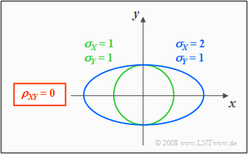
If the components $X$ and $Y$ are uncorrelated $(ρ_{XY} = 0)$, the equation obtained for the contour lines is:
- $$\frac{x^{\rm 2}}{\sigma_{X}^{\rm 2}}+\frac{y^{\rm 2}}{\sigma_{Y}^{\rm 2}} =\rm const.$$
In this case, the contour lines describe the following figures:
- Circles (if $σ_X = σ_Y$, green curve), or
- Ellipses (for $σ_X ≠ σ_Y$, blue curve) in alignment of the two axes.
Regression line
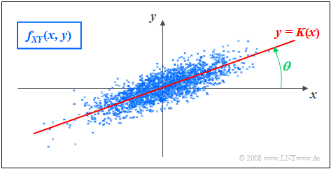
As regression line is called the straight line $y = K(x)$ in the $(x, y)$–plane through the "center" $(m_X, m_Y)$. This has the following properties:
- The mean square error from this straight line - viewed in $y$–direction and averaged over all $N$ measurement points - is minimal:
- $$\overline{\varepsilon_y^{\rm 2} }=\frac{\rm 1}{N} \cdot \sum_{\nu=\rm 1}^{N}\; \;\big [y_\nu - K(x_{\nu})\big ]^{\rm 2}={\rm minimum}.$$
- The correlation straight line can be interpreted as a kind of "statistical symmetry axis". The equation of the straight line in the general case is:
- $$y=K(x)=\frac{\sigma_Y}{\sigma_X}\cdot\rho_{XY}\cdot(x - m_X)+m_Y.$$
- The angle that the correlation line makes to the $x$–axis is:
- $$\theta={\rm arctan}(\frac{\sigma_{Y} }{\sigma_{X} }\cdot \rho_{XY}).$$
For correlated components $(ρ_{XY} ≠ 0)$ the contour lines of the PDF are (almost) always elliptic, so also for the special case $σ_X = σ_Y$.
Exception: $ρ_{XY}=\pm 1$ ⇒ "Dirac-wall"; see "Exercise 4.4" in the book "Stochastic Signal Theory", subtask (5).
Here, the determining equation of the PDF height lines is:
- $$f_{XY}(x, y) = {\rm const.} \hspace{0.5cm} \rightarrow \hspace{0.5cm} \frac{x^{\rm 2} }{\sigma_{X}^{\rm 2}}+\frac{y^{\rm 2} }{\sigma_{Y}^{\rm 2} }-{\rm 2}\cdot\rho_{XY}\cdot\frac{x\cdot y}{\sigma_X\cdot \sigma_Y}={\rm const.}$$
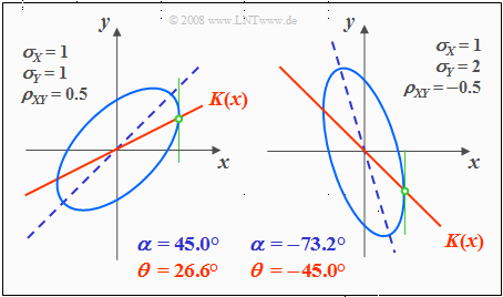
The graph shows a contour line in lighter blue for each of two different sets of parameters.
- The ellipse major axis is dashed in dark blue.
- The "regression line" $K(x)$ is drawn in red throughout.
Based on this plot, the following statements are possible:
- The ellipse shape depends not only on the correlation coefficient $ρ_{XY}$ but also on the ratio of the two standard deviations $σ_X$ and $σ_Y$ .
- The angle of inclination $α$ of the ellipse major axis (dashed straight line) with respect to the $x$–axis also depends on $σ_X$, $σ_Y$ and $ρ_{XY}$ :
- $$\alpha = {1}/{2} \cdot {\rm arctan } \big ( 2 \cdot \rho_{XY} \cdot \frac {\sigma_X \cdot \sigma_Y}{\sigma_X^2 - \sigma_Y^2} \big ).$$
- The (red) correlation line $y = K(x)$ of a Gaussian 2D-random variable always lies below the (blue dashed) ellipse major axis.
- $K(x)$ can be geometrically constructed from the intersection of the contour lines and their vertical tangents, as indicated in the sketch in green color.
Two dimensional cumulative distribution function ⇒ 2D–CDF
$\text{Definition:}$ The 2D cumulative distribution function like the 2D-CDF, is merely a useful extension of the "one-dimensional distribution function" (PDF):
- $$F_{XY}(x,y) = {\rm Pr}\big [(X \le x) \cap (Y \le y) \big ] .$$
The following similarities and differences between the "1D–CDF" and the" 2D–CDF" emerge:
- The functional relationship between "2D–PDF" and "2D–CDF" is given by the integration as in the one-dimensional case, but now in two dimensions. For continuous random variables, the following holds:
- $$F_{XY}(x,y)=\int_{-\infty}^{y} \int_{-\infty}^{x} f_{XY}(\xi,\eta) \,\,{\rm d}\xi \,\, {\rm d}\eta .$$
- Inversely, the probability density function can be given from the cumulative distribution function by partial differentiation to $x$ and $y$ :
- $$f_{XY}(x,y)=\frac{{\rm d}^{\rm 2} F_{XY}(\xi,\eta)}{{\rm d} \xi \,\, {\rm d} \eta}\Bigg|_{\left.{x=\xi \atop {y=\eta}}\right.}.$$
- In terms of the cumulative distribution function $F_{XY}(x, y)$ the following limits apply:
- $$F_{XY}(-\infty,\ -\infty) = 0,\hspace{0.5cm}F_{XY}(x,\ +\infty)=F_{X}(x ),\hspace{0.5cm} F_{XY}(+\infty,\ y)=F_{Y}(y ) ,\hspace{0.5cm}F_{XY}(+\infty,\ +\infty) = 1.$$
- In the limiting case $($infinitely large $x$ and $y)$ thus the value $1$ is obtained for the "2D–CDF". From this we obtain the normalization condition for the two-dimensional probability density function:
- $$\int_{-\infty}^{+\infty} \int_{-\infty}^{+\infty} f_{XY}(x,y) \,\,{\rm d}x \,\,{\rm d}y=1 . $$
$\text{Conclusion:}$ Note the significant difference between one-dimensional and two-dimensional random variables:
- For one-dimensional random variables, the area under the PDF always yields $1$.
- For two-dimensional random variables, the PDF volume always equals $1$.
Exercises
- Select the number $(1,\ 2$, ... $)$ of the task to be processed. The number "0" corresponds to a "Reset": Setting as at the program start.
- A task description is displayed. Parameter values are adjusted. Solution after pressing "Sample solution".
- In the task description, we use $\rho$ instead of $\rho_{XY}$.
- For the one-dimensional Gaussian PDF holds: $f_{X}(x) = \sqrt{1/(2\pi \cdot \sigma_X^2)} \cdot {\rm e}^{-x^2/(2 \hspace{0.05cm}\cdot \hspace{0.05cm} \sigma_X^2)}$.
(1) Get familiar with the program using the default $(\sigma_X=1, \ \sigma_Y=0.5, \ \rho = 0.7)$. Interpret the graphs for $\rm PDF$ and $\rm CDF$.
- $\rm PDF$ is a ridge with the maximum at $x = 0, \ y = 0$. The ridge is slightly twisted with respect to the $x$–axis.
- $\rm CDF$ is obtained from $\rm PDF$ by continuous integration in both directions. The maximum $($near $1)$ occurs at $x=3, \ y=3$.
(2) The new setting is $\sigma_X= \sigma_Y=1, \ \rho = 0$. What are the values for $f_{XY}(0,\ 0)$ and $F_{XY}(0,\ 0)$? Interpret the results
- The PDF maximum is $f_{XY}(0,\ 0) = 1/(2\pi)= 0.1592$, because of $\sigma_X= \sigma_Y = 1, \ \rho = 0$. The contour lines are circles.
- For the CDF value: $F_{XY}(0,\ 0) = [{\rm Pr}(X \le 0)] \cdot [{\rm Pr}(Y \le 0)] = 0.25$. Minor deviation due to numerical integration.
(3) The settings of $(2)$ continue to apply. What are the values for $f_{XY}(0,\ 1)$ and $F_{XY}(0,\ 1)$? Interpret the results.
- It holds $f_{XY}(0,\ 1) = f_{X}(0) \cdot f_{Y}(1) = [ \sqrt{1/(2\pi)}] \cdot [\sqrt{1/(2\pi)} \cdot {\rm e}^{-0.5}] = 1/(2\pi) \cdot {\rm e}^{-0.5} = 0.0965$.
- The program returns $F_{XY}(0,\ 1) = [{\rm Pr}(X \le 0)] \cdot [{\rm Pr}(Y \le 1)] = 0.4187$, i.e. a larger value than in $(2)$, since it integrates over a wider range.
(4) The settings are kept. What values are obtained for $f_{XY}(1,\ 0)$ and $F_{XY}(1,\ 0)$? Interpret the results
- Due to rotational symmetry, same results as in $(3)$.
(5) Is the statement true: "Elliptic contour lines exist only for $\rho \ne 0$". Interpret the $\rm 2D\hspace{-0.1cm}-\hspace{-0.1cm}PDF$ and $\rm 2D\hspace{-0.1cm}-\hspace{-0.1cm}CDF$ for $\sigma_X=1, \ \sigma_Y=0.5$ and $\rho = 0$.
- No! Also, for $\ \rho = 0$ the contour lines are elliptical (not circular) if $\sigma_X \ne \sigma_Y$.
- For $\sigma_X \gg \sigma_Y$ the $\rm 2D\hspace{-0.1cm}-\hspace{-0.1cm}PDF$ has the shape of an elongated ridge parallel to $x$–axis, for $\sigma_X \ll \sigma_Y$ parallel to $y$–axis.
- For $\sigma_X \gg \sigma_Y$ the slope of $\rm 2D\hspace{-0.1cm}-\hspace{-0.1cm}CDF$ in the direction of the $y$–axis is much steeper than in the direction of the $x$–axis.
(6) Starting from $\sigma_X=\sigma_Y=1\ \rho = 0.7$ vary the correlation coefficient $\rho$. What is the slope angle $\alpha$ of the ellipse main axis?
- For $\rho > 0$: $\alpha = 45^\circ$. For $\rho < 0$: $\alpha = -45^\circ$. For $\rho = 0$: The contour lines are circular and thus there are no ellipses main axis.
(7) Starting from $\sigma_X=\sigma_Y=1\ \rho = 0.7$ vary the correlation coefficient $\rho$. What is the slope angle $\theta$ of the correlation line $K(x)$?
- For $\sigma_X=\sigma_Y$: $\theta={\rm arctan}\ (\rho)$. The slope increases with increasing $\rho > 0$. In all cases, $\theta < \alpha = 45^\circ$ holds. For $\rho = 0.7$ this gives $\theta = 35^\circ$.
(8) Starting from $\sigma_X=\sigma_Y=0.75, \ \rho = 0.7$ vary the parameters $\sigma_Y$ and $\rho $. What statements hold for the angles $\alpha$ and $\theta$?
- For $\sigma_Y<\sigma_X$: $\alpha < 45^\circ$. For $\sigma_Y>\sigma_X$: $\alpha > 45^\circ$. For all settings: The correlation line is below the ellipse main axis.
(9) Assume $\sigma_X= 1, \ \sigma_Y=0.75, \ \rho = 0.7$. Vary $\rho$. How to construct the correlation line from the contour lines?
- The correlation line intersects all contour lines at that points where the tangent line is perpendicular to the contour line.
(10) Now let be $\sigma_X= \sigma_Y=1, \ \rho = 0.95$. Interpret the $\rm 2D\hspace{-0.1cm}-\hspace{-0.1cm}PDF$. Which statements are true for the limiting case $\rho \to 1$ ?
- The $\rm 2D\hspace{-0.1cm}-\hspace{-0.1cm}WDF$ only has components near the ellipse main axis. The correlation line is just below: $\alpha = 45^\circ, \ \theta = 43.5^\circ$.
- In the limiting case $\rho \to 1$ it holds $\theta = \alpha = 45^\circ$. Outside the correlation line, the $\rm 2D\hspace{-0.1cm}-\hspace{-0.1cm}PDF$ would have no shares. That is:
- Along the correlation line, there would be a "Dirac wall" ⇒ All values are infinitely large, nevertheless Gaussian weighted around the mean.
Applet Manual
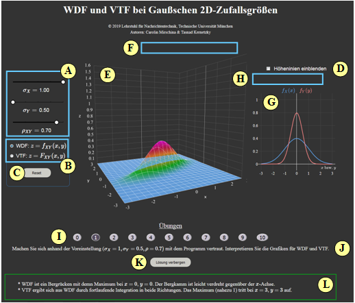
(A) Parameter input via slider: $\sigma_X$, $\sigma_Y$ and $\rho$.
(B) Selection: Representation of PDF or CDF.
(C) Reset: Setting as at program start.
(D) Display contour lines instead of one-dimensional PDF.
(E) Display range for two-dimensional PDF.
(F) Manipulation of the three-dimensional graph (zoom, rotate, ...)
(G) Display range for "one-dimensional PDF" or "contour lines".
(H) Manipulation of the two-dimensional graphics ("one-dimensional PDF")
( I ) Area for exercises: Task selection.
(J) Area for exercises: Task description
(K) Area for exercises: Show/hide solution
( L) Area for exercises: Output of the sample solution
Note: Value output of the graphics $($both 2D and 3D$)$ via mouse control.
About the Authors
This interactive calculation tool was designed and implemented at the Institute for Communications Engineering at the Technical University of Munich.
- The first version was created in 2003 by Ji Li as part of his diploma thesis with “FlashMX – Actionscript” (Supervisor: Günter Söder).
- In 2019 the program was redesigned by Carolin Mirschina as part of her bachelor thesis (Supervisor: Tasnád Kernetzky ) via "HTML5".
- Last revision and English version 2021 by Carolin Mirschina in the context of a working student activity.
The conversion of this applet to HTML 5 was financially supported by "Studienzuschüsse" (Faculty EI of the TU Munich). We thank.


