Difference between revisions of "Aufgaben:Exercise 2.5: Residual Redundancy with LZW Coding"
| Line 109: | Line 109: | ||
===Solution=== | ===Solution=== | ||
{{ML-Kopf}} | {{ML-Kopf}} | ||
| − | '''(1)''' | + | '''(1)''' The approximation $r\hspace{0.05cm}'(N)$ agrees exactly by definition for the sequence length $N = 10000$ with the residual redundancy $r(N) = 0.265$ determined by simulation. |
| − | * | + | *Thus |
:$$A = 4 \cdot r(N = 10000) =4 \cdot {0.265} \hspace{0.15cm}\underline{= 1.06} | :$$A = 4 \cdot r(N = 10000) =4 \cdot {0.265} \hspace{0.15cm}\underline{= 1.06} | ||
\hspace{0.05cm}. $$ | \hspace{0.05cm}. $$ | ||
| Line 116: | Line 116: | ||
| − | '''(2)''' | + | '''(2)''' From the relationship ${A}/{\rm lg}\hspace{0.1cm}(N) ≤ 0.05$ ⇒ ${A}/{\rm lg}\hspace{0.1cm}(N) = 0.05$ it follows: |
:$${{\rm lg}\hspace{0.1cm}N_{\rm 2}} = \frac{A}{0.05} = 21.2 \hspace{0.3cm}\Rightarrow\hspace{0.3cm} | :$${{\rm lg}\hspace{0.1cm}N_{\rm 2}} = \frac{A}{0.05} = 21.2 \hspace{0.3cm}\Rightarrow\hspace{0.3cm} | ||
N_{\rm 2} = 10^{21.2} \hspace{0.15cm}\underline{= 1.58 \cdot 10^{21}} | N_{\rm 2} = 10^{21.2} \hspace{0.15cm}\underline{= 1.58 \cdot 10^{21}} | ||
| Line 123: | Line 123: | ||
| − | '''(3)''' | + | '''(3)''' In general, $r(N) = 1 - {H}/{K(N)} \hspace{0.05cm}.$ |
| − | *$\rm BQ1$ | + | *$\rm BQ1$ has entropy $H = 0.5$ bit/symbol. |
| − | * | + | *It follows that because $r(N) ≈ r\hspace{0.05cm}'(N)$ für $K(N_3) = 0.6$: |
:$$r(N_{\rm c}) = 1 - \frac{0.5}{0.6} = 0.167 \hspace{0.1cm}\Rightarrow\hspace{0.1cm} | :$$r(N_{\rm c}) = 1 - \frac{0.5}{0.6} = 0.167 \hspace{0.1cm}\Rightarrow\hspace{0.1cm} | ||
{\rm lg}\hspace{0.1cm}N_{\rm 3} = \frac{A}{0.167} = 6.36 | {\rm lg}\hspace{0.1cm}N_{\rm 3} = \frac{A}{0.167} = 6.36 | ||
| Line 134: | Line 134: | ||
| − | [[File:EN_Inf_A_2_5d_v2.png|right|frame| | + | [[File:EN_Inf_A_2_5d_v2.png|right|frame|Results for $\rm BQ2$]] |
| − | '''(4)''' | + | '''(4)''' For $N = 10000$ gilt $r(N) ≈ r\hspace{0.05cm}'(N) = 0.19$: |
:$$\frac{A}{{\rm lg}\hspace{0.1cm}10000} = 0.19 \hspace{0.3cm}\Rightarrow\hspace{0.3cm} | :$$\frac{A}{{\rm lg}\hspace{0.1cm}10000} = 0.19 \hspace{0.3cm}\Rightarrow\hspace{0.3cm} | ||
A = 0.19 \cdot 4 = 0.76 \hspace{0.05cm}. $$ | A = 0.19 \cdot 4 = 0.76 \hspace{0.05cm}. $$ | ||
| − | * | + | *The results are summarised in the table opposite. |
| − | * | + | *One can see the very good agreement between $r(N)$ and $r\hspace{0.05cm}'(N)$. |
| − | * | + | *The numerical values sought are marked in red in the table: |
$$r'(N = 50000)\hspace{0.15cm}\underline{ = 0.162},\hspace{0.3cm}r'(N = 10^{6})\hspace{0.15cm}\underline{ = 0.127},\hspace{0.3cm} | $$r'(N = 50000)\hspace{0.15cm}\underline{ = 0.162},\hspace{0.3cm}r'(N = 10^{6})\hspace{0.15cm}\underline{ = 0.127},\hspace{0.3cm} | ||
r'(N = 10^{12})\hspace{0.15cm}\underline{ = 0.063}.$$ | r'(N = 10^{12})\hspace{0.15cm}\underline{ = 0.063}.$$ | ||
| − | * | + | *For the compression factor, (the apostrophe indicates that the approximation $r\hspace{0.05cm}'(N)$ was assumed): |
:$$K\hspace{0.05cm}'(N) = \frac{1}{1 - r\hspace{0.05cm}'(N)}\hspace{0.05cm}.$$ | :$$K\hspace{0.05cm}'(N) = \frac{1}{1 - r\hspace{0.05cm}'(N)}\hspace{0.05cm}.$$ | ||
| − | * | + | *Thus, for the length of the LZW output string: |
:$$L\hspace{0.05cm}'(N) = K\hspace{0.05cm}'(N) \cdot N = \frac{N}{1 - r\hspace{0.05cm}'(N)}\hspace{0.05cm}.$$ | :$$L\hspace{0.05cm}'(N) = K\hspace{0.05cm}'(N) \cdot N = \frac{N}{1 - r\hspace{0.05cm}'(N)}\hspace{0.05cm}.$$ | ||
| − | [[File:EN_Inf_A_2_5e_v2.png|right|frame| | + | [[File:EN_Inf_A_2_5e_v2.png|right|frame|Results for $\rm BQ3$]] |
| − | '''(5)''' | + | '''(5)''' Following a similar procedure as in subtask '''(4)''' we obtain the fitting parameter $\rm BQ3$ for the binary source $A = 1.36$ and from this the results according to the table with a blue background. |
| − | <u> | + | <u>Hint:</u> The last column of this table is only understandable with knowledge of subtask '''(6)''' . There it is shown that the source $\rm BQ3$ has the entropy $H = 0.25$ bit/source symbol. |
| − | *In | + | *In this case, the following applies to the compression factor: |
:$$K\hspace{0.05cm}'(N) = \frac{H}{1 - r\hspace{0.05cm}'(N)} = \frac{0.25}{1 - r'(N)} \hspace{0.05cm}.$$ | :$$K\hspace{0.05cm}'(N) = \frac{H}{1 - r\hspace{0.05cm}'(N)} = \frac{0.25}{1 - r'(N)} \hspace{0.05cm}.$$ | ||
| − | * | + | *Thus, for the values of residual redundancy we are looking for, we obtain: |
:$$r\hspace{0.05cm}'(N = 50000)\hspace{0.15cm}\underline{ = 0.289},\hspace{0.3cm}r\hspace{0.05cm}'(N = 10^{6})\hspace{0.15cm}\underline{ = 0.227},\hspace{0.3cm} | :$$r\hspace{0.05cm}'(N = 50000)\hspace{0.15cm}\underline{ = 0.289},\hspace{0.3cm}r\hspace{0.05cm}'(N = 10^{6})\hspace{0.15cm}\underline{ = 0.227},\hspace{0.3cm} | ||
r\hspace{0.05cm}'(N = 10^{12})\hspace{0.15cm}\underline{ = 0.113}.$$ | r\hspace{0.05cm}'(N = 10^{12})\hspace{0.15cm}\underline{ = 0.113}.$$ | ||
| − | * | + | *Thus, for $N = 10^{12}$ , the compression factor $(0.282)$ still deviates significantly from the entropy $(0.25)$ which can only be achieved for $N \to \infty$ (source coding theorem). |
| − | '''(6)''' | + | '''(6)''' The individual approximations $r\hspace{0.05cm}'(N)$ differ only by the parameter $A$. Here we found: |
| − | # | + | # Source $\rm BQ1$ with $H = 0.50$ ⇒ $A = 1.06$ ⇒ according to the specification sheet, |
| − | # | + | # Source $\rm BQ2$ with $H = 1.00$ ⇒ $A = 0.76$ ⇒ see subtask '''(4)''', |
| − | # | + | # Source $\rm BQ3$ $(H$ unknown$)$: $A = 4 · 0.34 =1.36$ ⇒ corresponding to the last column in the table. |
| − | * | + | *Obviously, the smaller the entropy $H$ the larger the adjustment factor $A$ (and vice versa). |
| − | * | + | *Since exactly one solution is possible, $H = 0.25$ bit/source symbol must be correct ⇒ <u>answer 4</u>. |
| − | * | + | *In fact, the probabilities $p_{\rm A} = 0.96$ and $p_{\rm B} = 0.04$ ⇒ $H ≈ 0.25$ were used in the simulation for source $\rm BQ3$ . |
{{ML-Fuß}} | {{ML-Fuß}} | ||
Revision as of 20:35, 31 July 2021
We assume here a binary input sequence of length $N$ and consider three different binary message sources:
- $\rm BQ1$: Symbol probabilities $p_{\rm A} = 0.89$ and $p_{\rm B} = 0.11$, i.e. different
⇒ entropy $H = 0.5\text{ bit/source symbol}$ ⇒ the source is redundant. - $\rm BQ2$: $p_{\rm A} = p_{\rm B} = 0.5$ (equally probable)
⇒ entropy $H = 1\text{ bit/source symbol}$ ⇒ the source is redundancy-free. - $\rm BQ3$: There is no concrete information on the statistics here.
In subtask (6) you are to estimate the entropy $H$ of this source.
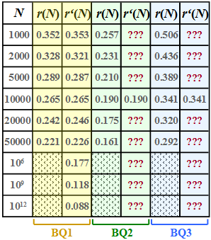
For these three sources, the respective residual redundancy $r(N)$ was determined by simulation, which remains in the binary sequence after Lempel–Ziv–Welch–coding in der Binärfolge verbleibt.
The results are shown in the first column of the above table for the sources
- $\rm BQ1$ (yellow background),
- $\rm BQ2$ (green background) and
- $\rm BQ3$ (blue background)
whereby we have restricted ourselves to sequence lengths $N ≤ 50000$ in the simulation.
The relative redundancy of the output sequence – simplified called residual redundancy – can be calculated from
- the length $N$ of the input sequence,
- the length $L(N)$ of the output sequence and
- the entropy $H$
can be calculated in the following way:
- $$r(N) = \frac{L(N) - N \cdot H}{L(N)}= 1 - \frac{ N \cdot H}{L(N)}\hspace{0.05cm}.$$
This takes into account that with perfect source coding the length of the output sequence could be lowered to the value $L_{\rm min} = N · H$ .
- With non-perfect source coding, $L(n) - N · H$ gives the remaining redundancy (with the pseudo–unit "bit").
- After dividing by $L(n)$ , one obtains the relative redundancy $r(n)$ with the value range between zero and one; $r(n)$ should be as small as possible.
A second parameter for measuring the efficiency of LZW coding is the compression factor $K(N)$, which should also be small as the quotient of the lengths of the output and input sequences:
- $$K(N) = {L(N) }/{N} \hspace{0.05cm},$$
In the theory section it was shown that the residual redundancy $r(n)$ is often given by the function
- $$r\hspace{0.05cm}'(N) =\frac {A}{{\rm lg}\hspace{0.1cm}(N)} \hspace{0.5cm}{\rm mit}\hspace{0.5cm} A = 4 \cdot {r(N = 10000)} \hspace{0.05cm}.$$
is well approximated.
- This approximation $r\hspace{0.05cm}'(N)$ is given for $\rm BQ1$ in the second column of the table above.
- In subtasks (4) and (5) you are to make the approximation for sources $\rm BQ2$ and $\rm BQ3$ .
Hints:
- The task belongs to the chapter Compression according to Lempel, Ziv and Welch.
- In particular, reference is made to the pages
- The descriptive variables $K(N)$ and $r(N)$ are deterministically related.
Questions
Solution
- Thus
- $$A = 4 \cdot r(N = 10000) =4 \cdot {0.265} \hspace{0.15cm}\underline{= 1.06} \hspace{0.05cm}. $$
(2) From the relationship ${A}/{\rm lg}\hspace{0.1cm}(N) ≤ 0.05$ ⇒ ${A}/{\rm lg}\hspace{0.1cm}(N) = 0.05$ it follows:
- $${{\rm lg}\hspace{0.1cm}N_{\rm 2}} = \frac{A}{0.05} = 21.2 \hspace{0.3cm}\Rightarrow\hspace{0.3cm} N_{\rm 2} = 10^{21.2} \hspace{0.15cm}\underline{= 1.58 \cdot 10^{21}} \hspace{0.05cm}.$$
(3) In general, $r(N) = 1 - {H}/{K(N)} \hspace{0.05cm}.$
- $\rm BQ1$ has entropy $H = 0.5$ bit/symbol.
- It follows that because $r(N) ≈ r\hspace{0.05cm}'(N)$ für $K(N_3) = 0.6$:
- $$r(N_{\rm c}) = 1 - \frac{0.5}{0.6} = 0.167 \hspace{0.1cm}\Rightarrow\hspace{0.1cm} {\rm lg}\hspace{0.1cm}N_{\rm 3} = \frac{A}{0.167} = 6.36 \hspace{0.1cm}\Rightarrow\hspace{0.1cm} N_{\rm 3} = 10^{6.36} \hspace{0.15cm}\underline{= 2.29 \cdot 10^{6}} \hspace{0.05cm}.$$
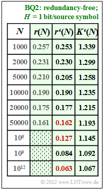
(4) For $N = 10000$ gilt $r(N) ≈ r\hspace{0.05cm}'(N) = 0.19$:
- $$\frac{A}{{\rm lg}\hspace{0.1cm}10000} = 0.19 \hspace{0.3cm}\Rightarrow\hspace{0.3cm} A = 0.19 \cdot 4 = 0.76 \hspace{0.05cm}. $$
- The results are summarised in the table opposite.
- One can see the very good agreement between $r(N)$ and $r\hspace{0.05cm}'(N)$.
- The numerical values sought are marked in red in the table:
$$r'(N = 50000)\hspace{0.15cm}\underline{ = 0.162},\hspace{0.3cm}r'(N = 10^{6})\hspace{0.15cm}\underline{ = 0.127},\hspace{0.3cm} r'(N = 10^{12})\hspace{0.15cm}\underline{ = 0.063}.$$
- For the compression factor, (the apostrophe indicates that the approximation $r\hspace{0.05cm}'(N)$ was assumed):
- $$K\hspace{0.05cm}'(N) = \frac{1}{1 - r\hspace{0.05cm}'(N)}\hspace{0.05cm}.$$
- Thus, for the length of the LZW output string:
- $$L\hspace{0.05cm}'(N) = K\hspace{0.05cm}'(N) \cdot N = \frac{N}{1 - r\hspace{0.05cm}'(N)}\hspace{0.05cm}.$$
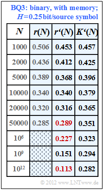
(5) Following a similar procedure as in subtask (4) we obtain the fitting parameter $\rm BQ3$ for the binary source $A = 1.36$ and from this the results according to the table with a blue background.
Hint: The last column of this table is only understandable with knowledge of subtask (6) . There it is shown that the source $\rm BQ3$ has the entropy $H = 0.25$ bit/source symbol.
- In this case, the following applies to the compression factor:
- $$K\hspace{0.05cm}'(N) = \frac{H}{1 - r\hspace{0.05cm}'(N)} = \frac{0.25}{1 - r'(N)} \hspace{0.05cm}.$$
- Thus, for the values of residual redundancy we are looking for, we obtain:
- $$r\hspace{0.05cm}'(N = 50000)\hspace{0.15cm}\underline{ = 0.289},\hspace{0.3cm}r\hspace{0.05cm}'(N = 10^{6})\hspace{0.15cm}\underline{ = 0.227},\hspace{0.3cm} r\hspace{0.05cm}'(N = 10^{12})\hspace{0.15cm}\underline{ = 0.113}.$$
- Thus, for $N = 10^{12}$ , the compression factor $(0.282)$ still deviates significantly from the entropy $(0.25)$ which can only be achieved for $N \to \infty$ (source coding theorem).
(6) The individual approximations $r\hspace{0.05cm}'(N)$ differ only by the parameter $A$. Here we found:
- Source $\rm BQ1$ with $H = 0.50$ ⇒ $A = 1.06$ ⇒ according to the specification sheet,
- Source $\rm BQ2$ with $H = 1.00$ ⇒ $A = 0.76$ ⇒ see subtask (4),
- Source $\rm BQ3$ $(H$ unknown$)$: $A = 4 · 0.34 =1.36$ ⇒ corresponding to the last column in the table.
- Obviously, the smaller the entropy $H$ the larger the adjustment factor $A$ (and vice versa).
- Since exactly one solution is possible, $H = 0.25$ bit/source symbol must be correct ⇒ answer 4.
- In fact, the probabilities $p_{\rm A} = 0.96$ and $p_{\rm B} = 0.04$ ⇒ $H ≈ 0.25$ were used in the simulation for source $\rm BQ3$ .


