Difference between revisions of "Aufgaben:Exercise 3.11Z: Metric and Accumutated Metric"
| Line 2: | Line 2: | ||
{{quiz-Header|Buchseite=Digital_Signal_Transmission/Viterbi_Receiver}} | {{quiz-Header|Buchseite=Digital_Signal_Transmission/Viterbi_Receiver}} | ||
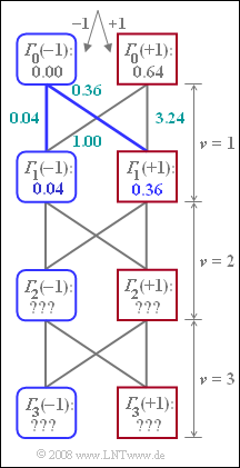
| − | [[File:P_ID1476__Dig_Z_3_11.png|right|frame|Calculation of the minimum | + | [[File:P_ID1476__Dig_Z_3_11.png|right|frame|Calculation of the minimum accumulated metrics]] |
| − | For the maximum likelihood constellation with bipolar amplitude coefficient $a_{\rm \nu} ∈ \{+1, –1\}$ discussed in [[Aufgaben:Exercise_3.11:_Viterbi_Receiver_and_Trellis_Diagram|"Exercise 3.11"]], | + | For the maximum likelihood constellation with bipolar amplitude coefficient $a_{\rm \nu} ∈ \{+1, –1\}$ discussed in [[Aufgaben:Exercise_3.11:_Viterbi_Receiver_and_Trellis_Diagram|"Exercise 3.11"]], the metrics $\varepsilon_{\rm \nu}(i)$ and the minimum accumulated metrics ${\it \Gamma}_{\rm \nu}(–1)$ and ${\it \Gamma}_{\rm \nu}(+1)$ are to be determined. |
| − | The basic pulse is given by the two values $g_0$ and $g_{\rm –1}$. These, as well as the detection samples $d_0$ and $d_1$, can be taken from the following calculations for the | + | The basic pulse is given by the two values $g_0$ and $g_{\rm –1}$. These, as well as the detection samples $d_0$ and $d_1$, can be taken from the following calculations for the metrics $\varepsilon_{\rm \nu}(i)$ at the times $\nu = 0$ and $\nu = 1$. Note that the symbol $a_0 = 0$ is always sent before the actual message $(a_1$, $a_2$, $a_3)$. |
For the time $\nu = 0$ holds: | For the time $\nu = 0$ holds: | ||
| Line 13: | Line 13: | ||
From this it could be concluded already at time $\nu = 0$ that with high probability $a_1 = -\hspace{-0.05cm}1$. | From this it could be concluded already at time $\nu = 0$ that with high probability $a_1 = -\hspace{-0.05cm}1$. | ||
| − | For time $\nu = 1$, the following | + | For time $\nu = 1$, the following metrics result: |
:$$\varepsilon_{1}(+1, +1) \ = \ \big[-0.8- 0.6 -0.4\big]^2=3.24 | :$$\varepsilon_{1}(+1, +1) \ = \ \big[-0.8- 0.6 -0.4\big]^2=3.24 | ||
\hspace{0.05cm},$$ | \hspace{0.05cm},$$ | ||
| Line 23: | Line 23: | ||
\hspace{0.05cm}.$$ | \hspace{0.05cm}.$$ | ||
| − | The minimum | + | The minimum accumulated metrics ${\it \Gamma}_{\rm \nu}(-\hspace{-0.07cm}1)$ and ${\it \Gamma}_{\rm \nu}(+1)$ that can be calculated with these six metrics are already plotted in the graph. The other detection samples are $d_{2}=0.1 \hspace{0.05cm},\hspace{0.1cm} |
d_{3}=0.5 \hspace{0.05cm}.$ | d_{3}=0.5 \hspace{0.05cm}.$ | ||
| Line 58: | Line 58: | ||
+ $±1.0.$ | + $±1.0.$ | ||
| − | {Give the minimum | + | {Give the minimum accumulated metrics for time $\nu = 2$ $(d_2 = 0.1)$. |
|type="{}"} | |type="{}"} | ||
${\it \Gamma}_2(+1)\ = \ $ { 0.13 3% } | ${\it \Gamma}_2(+1)\ = \ $ { 0.13 3% } | ||
${\it \Gamma}_2(-\hspace{-0.05cm}1)\ = \ $ { 0.37 3% } | ${\it \Gamma}_2(-\hspace{-0.05cm}1)\ = \ $ { 0.37 3% } | ||
| − | {Calculate the minimum | + | {Calculate the minimum accumulated metric for time $\nu = 3$ $(d_3 = 0.5)$. |
|type="{}"} | |type="{}"} | ||
${\it \Gamma}_3(+1) \ = \ $ { 0.38 3% } | ${\it \Gamma}_3(+1) \ = \ $ { 0.38 3% } | ||
| Line 74: | Line 74: | ||
| − | '''(2)''' The | + | '''(2)''' The metrics $\varepsilon_0(i)$ include the basic pulse value $g_{\rm –1}$, which is used to establish the relationship between the amplitude coefficient $a_1$ and the detection sample $d_0$ ($g_0$ is not included in these equations). |
*One can see $g_{\rm –1}\ \underline {= 0.4}$. | *One can see $g_{\rm –1}\ \underline {= 0.4}$. | ||
*From the equations for $\nu = 1$, the main value $g_0 \ \underline {= 0.6}$ can be read. | *From the equations for $\nu = 1$, the main value $g_0 \ \underline {= 0.6}$ can be read. | ||
| Line 87: | Line 87: | ||
| − | '''(4)''' The | + | '''(4)''' The metrics are obtained for $\nu = 2$ considering the result from (3) as follows: |
:$$\varepsilon_{2}(+1, +1) \ = \ [0.1 - 1.0]^2=0.81,\hspace{0.2cm} | :$$\varepsilon_{2}(+1, +1) \ = \ [0.1 - 1.0]^2=0.81,\hspace{0.2cm} | ||
\varepsilon_{2}(-1, +1) = [0.1 +0.2]^2=0.09 | \varepsilon_{2}(-1, +1) = [0.1 +0.2]^2=0.09 | ||
| Line 95: | Line 95: | ||
\hspace{0.05cm}.$$ | \hspace{0.05cm}.$$ | ||
| − | Thus, the minimum | + | Thus, the minimum accumulated metrics are: |
:$${\it \Gamma}_{2}(+1) \ = \ {\rm Min}\left[{\it \Gamma}_{1}(+1) + \varepsilon_{2}(+1, +1), | :$${\it \Gamma}_{2}(+1) \ = \ {\rm Min}\left[{\it \Gamma}_{1}(+1) + \varepsilon_{2}(+1, +1), | ||
\hspace{0.2cm}{\it \Gamma}_{1}(-1) + \varepsilon_{2}(-1, +1)\right] = | \hspace{0.2cm}{\it \Gamma}_{1}(-1) + \varepsilon_{2}(-1, +1)\right] = | ||
| Line 104: | Line 104: | ||
\hspace{0.05cm}.$$ | \hspace{0.05cm}.$$ | ||
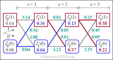
| − | [[File:P_ID1480__Dig_Z_3_11d.png|right|frame|Calculation of the minimum | + | [[File:P_ID1480__Dig_Z_3_11d.png|right|frame|Calculation of the minimum accumulated metrics]] |
<br>In the adjacent trellis diagram, the state "$1$" is to be interpreted as "$+1$" and "$0$" as "$–1$". | <br>In the adjacent trellis diagram, the state "$1$" is to be interpreted as "$+1$" and "$0$" as "$–1$". | ||
Revision as of 15:21, 4 July 2022
For the maximum likelihood constellation with bipolar amplitude coefficient $a_{\rm \nu} ∈ \{+1, –1\}$ discussed in "Exercise 3.11", the metrics $\varepsilon_{\rm \nu}(i)$ and the minimum accumulated metrics ${\it \Gamma}_{\rm \nu}(–1)$ and ${\it \Gamma}_{\rm \nu}(+1)$ are to be determined.
The basic pulse is given by the two values $g_0$ and $g_{\rm –1}$. These, as well as the detection samples $d_0$ and $d_1$, can be taken from the following calculations for the metrics $\varepsilon_{\rm \nu}(i)$ at the times $\nu = 0$ and $\nu = 1$. Note that the symbol $a_0 = 0$ is always sent before the actual message $(a_1$, $a_2$, $a_3)$.
For the time $\nu = 0$ holds:
- $$\varepsilon_{0}(+1) \ = \ \big[-0.4- 0.4\big]^2=0.64 \hspace{0.05cm},$$
- $$\varepsilon_{0}(-1) \ = \ \big[-0.4+ 0.4\big]^2=0.00 \hspace{0.05cm}.$$
From this it could be concluded already at time $\nu = 0$ that with high probability $a_1 = -\hspace{-0.05cm}1$.
For time $\nu = 1$, the following metrics result:
- $$\varepsilon_{1}(+1, +1) \ = \ \big[-0.8- 0.6 -0.4\big]^2=3.24 \hspace{0.05cm},$$
- $$\varepsilon_{1}(+1, -1) \ = \ \big[-0.8- 0.6 +0.4\big]^2=1.00 \hspace{0.05cm},$$
- $$\varepsilon_{1}(-1, +1) \ = \ \big[-0.8+ 0.6 -0.4\big]^2=0.36 \hspace{0.05cm},$$
- $$ \varepsilon_{1}(-1, -1) \ = \ \big[-0.8+ 0.6 +0.4\big]^2=0.04 \hspace{0.05cm}.$$
The minimum accumulated metrics ${\it \Gamma}_{\rm \nu}(-\hspace{-0.07cm}1)$ and ${\it \Gamma}_{\rm \nu}(+1)$ that can be calculated with these six metrics are already plotted in the graph. The other detection samples are $d_{2}=0.1 \hspace{0.05cm},\hspace{0.1cm} d_{3}=0.5 \hspace{0.05cm}.$
Notes:
- The exercise belongs to the chapter "Viterbi Receiver".
- All quantities are to be understood normalized here.
- Also assume bipolar and equal probability amplitude coefficients: ${\rm Pr} (a_\nu = -\hspace{-0.05cm}1) = {\rm Pr} (a_\nu = +1)= 0.5.$
- The topic is also covered in the interactive applet "Properties of the Viterbi Receiver".
Questions
Solution
(2) The metrics $\varepsilon_0(i)$ include the basic pulse value $g_{\rm –1}$, which is used to establish the relationship between the amplitude coefficient $a_1$ and the detection sample $d_0$ ($g_0$ is not included in these equations).
- One can see $g_{\rm –1}\ \underline {= 0.4}$.
- From the equations for $\nu = 1$, the main value $g_0 \ \underline {= 0.6}$ can be read.
(3) The correct solutions are 1 and 4:
- The possible useful samples are $\pm g_0 \pm g_{\rm –1} = \pm 0.6 \pm0.4$, i.e. $\underline {±0.2}$ and $\underline {±1.0}$.
- In contrast, unipolar signaling ⇒ $a_\nu \in \{0, \hspace{0.05cm} 1\}$ would result in values of $0, \ 0.4, \ 0.6$ and $1$.
- The relationship between bipolar values $b_i$ and unipolar equivalents $u_i$ is generally: $b_i = 2 \cdot u_i - 1 \hspace{0.05cm}.$
(4) The metrics are obtained for $\nu = 2$ considering the result from (3) as follows:
- $$\varepsilon_{2}(+1, +1) \ = \ [0.1 - 1.0]^2=0.81,\hspace{0.2cm} \varepsilon_{2}(-1, +1) = [0.1 +0.2]^2=0.09 \hspace{0.05cm},$$
- $$\varepsilon_{2}(+1, -1) \ = \ [0.1 -0.2]^2=0.01,\hspace{0.2cm} \varepsilon_{2}(-1, -1) = [0.1 +1.0]^2=1.21 \hspace{0.05cm}.$$
Thus, the minimum accumulated metrics are:
- $${\it \Gamma}_{2}(+1) \ = \ {\rm Min}\left[{\it \Gamma}_{1}(+1) + \varepsilon_{2}(+1, +1), \hspace{0.2cm}{\it \Gamma}_{1}(-1) + \varepsilon_{2}(-1, +1)\right] = {\rm Min}\left[0.36 + 0.81, 0.04 + 0.09\right]\hspace{0.15cm}\underline {= 0.13} \hspace{0.05cm},$$
- $${\it \Gamma}_{2}(-1) \ = \ {\rm Min}\left[{\it \Gamma}_{1}(+1) + \varepsilon_{2}(+1, -1), \hspace{0.2cm}{\it \Gamma}_{1}(-1) + \varepsilon_{2}(-1, -1)\right] = {\rm Min}\left[0.36 + 0.01, 0.04 + 1.21\right]\hspace{0.15cm}\underline {= 0.37} \hspace{0.05cm}.$$
In the adjacent trellis diagram, the state "$1$" is to be interpreted as "$+1$" and "$0$" as "$–1$".
Then holds:
- ${\it \Gamma}_2(+1) = 0.13$ is the minimum total error quantity under the hypothesis that the following symbol will be $a_3 = +1$.
- Under this assumption, $a_2 = \ –1$ is more likely than $a_2 = +1$, as shown in the trellis diagram (the incoming path is blue).
- A realistic alternative to the combination "$a_2 = \ –1, a_3 = +1$" is "$a_2 = +1, a_3 = \ –1$", which lead to the minimum total error quantity ${\it \Gamma}_2(–1) = 0.37$. Here, the incoming path is red.
(5) For time $\nu = 3$, the following equations hold:
- $$\varepsilon_{3}(+1, +1) \ = \ [0.5 - 1.0]^2=0.25,\hspace{0.2cm} \varepsilon_{3}(-1, +1) = [0.5 +0.2]^2=0.49 \hspace{0.05cm},$$
- $$\varepsilon_{3}(+1, -1) \ = \ [0.5 -0.2]^2=0.09,\hspace{0.2cm} \varepsilon_{3}(-1, -1) = [0.5 +1.0]^2=2.25 \hspace{0.05cm}.$$
- $$\Rightarrow \hspace{0.3cm}{\it \Gamma}_{3}(+1) \ = \ {\rm Min}\left[0.13 + 0.25, 0.37 + 0.49\right]\hspace{0.15cm}\underline {= 0.38} \hspace{0.05cm},\hspace{0.8cm} {\it \Gamma}_{3}(-1) \ = \ {\rm Min}\left[0.13 + 0.09, 0.37 + 2.25\right]\hspace{0.15cm}\underline {= 0.22} \hspace{0.05cm}.$$
- In both equations, the first term in each case is the smaller, with ${\it \Gamma}_2(+1) = 0.13$ included in each case.
- Therefore, the Viterbi receiver will certainly output $a_3 = +1$, no matter what information it will still get at later times ($\nu > 3$).
If we follow the continuous path in the trellis diagram, the other amplitude coefficients are also fixed by fixing $a_3 = +1$:
- $$a_1 = a_2 = \ –1.$$

