Difference between revisions of "Aufgaben:Exercise 3.4: Characteristic Function"
From LNTwww
(Die Seite wurde neu angelegt: „ {{quiz-Header|Buchseite=Stochastische Signaltheorie/*Kapitel* }} right| :Gegeben seien hier die drei Zufallsgrößen <i>x</i…“) |
|||
| (18 intermediate revisions by 4 users not shown) | |||
| Line 1: | Line 1: | ||
| − | {{quiz-Header|Buchseite= | + | {{quiz-Header|Buchseite=Theory_of_Stochastic_Signals/Expected_Values_and_Moments |
}} | }} | ||
| − | [[File:P_ID619__Sto_A_3_4.png|right|]] | + | [[File:P_ID619__Sto_A_3_4.png|right|frame|Rectangular and trapezoidal PDF]] |
| − | + | Given here are three random variables $x$, $y$ and $z$, mostly by their respective probability density functions: | |
| − | :* | + | *Nothing else is known about the random variable $x$: This can be both a discrete or a continuous random variable, and can have any PDF $f_x(x)$ The mean is generally equal $m_x$. |
| + | *The continuous random variable $y$ can take values in the range between $1$ to $3$ with equal probability. Mean: $m_y = 2.$ | ||
| + | *The random variable $z$ has the following characteristic function: | ||
| + | :$$C_z ({\it \Omega} ) = {\mathop{\rm si}\nolimits}( {3{\it \Omega}} ) \cdot {\mathop{\rm si}\nolimits} ( {2{\it \Omega} } ).$$ | ||
| + | :Besides, the qualitative course of the WDF $f_z(z)$ according to the blue sketch is assumed to be known. To be determined are the PDF parameters $a$, $b$, $c$ of this PDF. | ||
| − | |||
| − | |||
| − | |||
| − | |||
| − | |||
| − | : | + | Hints: |
| − | :$$ | + | *This exercise belongs to the chapter [[Theory_of_Stochastic_Signals/Expected_Values_and_Moments|Expected values and moments]]. |
| + | *Reference is made to the section [[Theory_of_Stochastic_Signals/Expected_Values_and_Moments#Characteristic_function|Charakteristic funcion]] . | ||
| + | |||
| + | *The characteristic function of a between $\pm a$ uniformly distributed random variable $z$ is: | ||
| + | :$$C ( {\it \Omega} ) = {\mathop{\rm si}\nolimits} ( {a {\it \Omega} } )\quad {\rm{with}}\quad {\mathop{\rm si}\nolimits}( x ) = \sin ( x )/x.$$ | ||
| − | === | + | ===Questions=== |
<quiz display=simple> | <quiz display=simple> | ||
| − | { | + | {Which statements are valid with respect to the characteristic function $C_x ( {\it \Omega} )$ always – that is, at any PDF ? |
|type="[]"} | |type="[]"} | ||
| − | - | + | - $C_x ( {\it \Omega} )$ is the Fourier transform of $f_x(x)$. |
| − | + | + | + The real part of $C_x ( {\it \Omega} )$ is an even function in ${\it \Omega}$. |
| − | + | + | + The imaginary part of $C_x ( {\it \Omega} )$ is an odd function in ${\it \Omega}$. |
| − | + | + | + The value at location ${\it \Omega} = 0$ is always $C_x ( {\it \Omega} ) = 1$. |
| − | - | + | - For a zero mean random variable $(m_x = 0)$ ⇒ $C_x ( {\it \Omega} )$ is always real. |
| − | { | + | {Calculate the characteristic function $C_y( {\it \Omega} )$. What are the real and imaginary parts at ${\it \Omega} = \pi/2$? |
|type="{}"} | |type="{}"} | ||
| − | $Re[C_y(\ | + | ${\rm Re}\big[C_y(\Omega\ =\ \pi/2)\big] \ = \ $ { -0.657--0.617 } |
| − | $Im[C_y(\ | + | ${\rm Im}\big[C_y(\Omega\ =\ \pi/2)\big] \ = \ $ { 0. } |
| − | { | + | {Determine the characteristic parameters $a$, $b$ and $c$ of the PDF $f_z(z)$. |
|type="{}"} | |type="{}"} | ||
| − | $a$ | + | $a \ = \ $ { 1 3% } |
| − | $b$ | + | $b \ = \ $ { 5 3% } |
| − | $c$ | + | $c \ = \ $ { 0.167 3% } |
| − | |||
</quiz> | </quiz> | ||
| − | === | + | ===Solutions=== |
{{ML-Kopf}} | {{ML-Kopf}} | ||
| − | + | '''(1)''' Correct are <u>the proposed solutions 2, 3 and 4</u>: | |
| − | :$$C_x( {\it \Omega | + | * $C_x( {\it \Omega} )$ is not the Fourier transform to $f_x(x)$, but the inverse Fourier transform: |
| + | :$$C_x( {\it \Omega } ) = \int_{ - \infty }^{ + \infty } {f_x }( x )\cdot {\rm{e}}^{\hspace{0.03cm}{\rm{j}}\hspace{0.05cm}\cdot \hspace{0.05cm}{\it \Omega\hspace{0.05cm}\cdot \hspace{0.05cm} x}} \hspace{0.1cm}{\rm{d}}x .$$ | ||
| + | *Also for this, the real part is always even and the imaginary part odd. For ${\it \Omega} = 0$ holds: | ||
| + | :$$C_x( {\it \Omega} = 0 ) = \int_{ - \infty }^{ + \infty } {f_x }( x ) \hspace{0.1cm}{\rm{d}}x = 1.$$ | ||
| + | *The last alternative does not always hold: A two-point distributed random variable $x \in \{-1, +3\}$ with probabilities $0.75$ and $0.25$ is zero mean $(m_x = 0)$, but has still a complex characteristic function. | ||
| − | |||
| − | |||
| − | |||
| − | + | '''(2)''' According to the general definition: | |
| − | :$$C_y( {\it \Omega } ) = \int_{ - \infty }^{ + \infty } {f_y }( y )\cdot {\rm{e}}^{{\rm{j}}{\it \Omega y}} \hspace{0.1cm}{\rm{d}}y = 0.5\int_1^3 {{\rm{e}}^{{\rm{j}}\Omega y} \hspace{0.1cm}{\rm{d}}y.} $$ | + | :$$C_y( {\it \Omega } ) = \int_{ - \infty }^{ + \infty } {f_y }( y )\cdot {\rm{e}}^{{\rm{j}}\hspace{0.05cm}\cdot \hspace{0.05cm}{\it \Omega\hspace{0.01cm}\hspace{0.05cm}\cdot \hspace{0.05cm} y}} \hspace{0.1cm}{\rm{d}}y = 0.5\int_1^3 {{\rm{e}}^{{\rm{j}}\hspace{0.05cm}\cdot \hspace{0.05cm}\Omega\hspace{0.05cm}\cdot \hspace{0.05cm} y} \hspace{0.1cm}{\rm{d}}y.} $$ |
| − | + | *After solving this integral, we get: | |
| − | :$$C_y ( {\it \Omega } ) = \frac{{{\rm{e}}^{{\rm{j}}3{\it \Omega } } - {\rm{e}}^{{\rm{j}}{\it \Omega } } }}{{2{\rm{j}}{\it \Omega } }} = \frac{{{\rm{e}}^{{\rm{j}}{\it \Omega } } - {\rm{e}}^{{\rm{ - j}}{\it \Omega }} }}{{2{\rm{j}}{\it \Omega } }} \cdot {\rm{e}}^{{\rm{ | + | :$$C_y ( {\it \Omega } ) = \frac{{{\rm{e}}^{{\rm{j}}\hspace{0.05cm}\cdot \hspace{0.05cm}3{\it \Omega } } - {\rm{e}}^{{\rm{j}}\hspace{0.05cm}\cdot \hspace{0.05cm}{\it \Omega } } }}{{2{\rm{j}}{\it \Omega } }} = = \frac{{{\rm{e}}^{{\rm{j}}\hspace{0.05cm}\cdot \hspace{0.05cm}{\it \Omega } } - {\rm{e}}^{{\rm{ - j}}\hspace{0.05cm}\cdot \hspace{0.05cm}{\it \Omega }} }}{{2{\rm{j}}{\it \Omega } }} \cdot {\rm{e}}^{{\rm{j\hspace{0.05cm}\cdot \hspace{0.05cm}2}}{\it \Omega } } .$$ |
| − | + | *Using Euler's theorem, this can also be written: | |
| − | :$$C_y ( {\it \Omega } ) = \frac{{\sin ( {\it \Omega } )}}{{\it \Omega } } \cdot {\rm{e}}^{{\rm{j2}}{\it \Omega } } .$$ | + | :$$C_y ( {\it \Omega } ) = \frac{{\sin ( {\it \Omega } )}}{{\it \Omega } } \cdot {\rm{e}}^{{\rm{j2}}\hspace{0.05cm}\cdot \hspace{0.05cm}{\it \Omega } } = {\rm si} ( {\it \Omega } ) \cdot {\rm{e}}^{{\rm{j2}}\hspace{0.05cm}\cdot \hspace{0.05cm}{\it \Omega } }.$$ |
| − | + | *For ${\it \Omega} = \pi/2$ we thus obtain a purely real numerical value: | |
:$${\rm Re}[C_y ({\it \Omega} = {\rm{\pi }}/2 )] = \frac{{\sin( {{\rm{\pi }}/2})}}{{{\rm{\pi }}/2}} \cdot {\rm{e}}^{{\rm{j\pi }}} = - \frac{2}{{\rm{\pi }}} | :$${\rm Re}[C_y ({\it \Omega} = {\rm{\pi }}/2 )] = \frac{{\sin( {{\rm{\pi }}/2})}}{{{\rm{\pi }}/2}} \cdot {\rm{e}}^{{\rm{j\pi }}} = - \frac{2}{{\rm{\pi }}} | ||
\hspace{0.15cm}\underline{\approx -0.637}, \hspace{0.5cm} | \hspace{0.15cm}\underline{\approx -0.637}, \hspace{0.5cm} | ||
{\rm Im}[C_y ({\it \Omega} = {\rm{\pi }}/2 )] \hspace{0.15cm}\underline{= 0} .$$ | {\rm Im}[C_y ({\it \Omega} = {\rm{\pi }}/2 )] \hspace{0.15cm}\underline{= 0} .$$ | ||
| − | + | ||
| − | [[File:P_ID620__Sto_A_3_4_c_neu.png| | + | '''(3)''' From the given correspondence it can be read that ${\rm si}(3 {\it \Omega} )$ is due to an between $\pm 3$ equally distributed random variable and ${\rm si}(2 {\it \Omega} )$ gives the transform of a uniform distribution between $\pm 2$. |
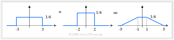
| − | + | [[File:P_ID620__Sto_A_3_4_c_neu.png|right|frame|Construction of the trapezoidal PDF]] | |
| + | *In the characteristic function, these two proportions are multiplicatively linked. | ||
| + | *Thus, the resulting PDF $f_z(z)$ is the convolution of these two rectangular functions. | ||
| + | *The three PDF parameters are thus: | ||
:$$\hspace{0.15cm}\underline{a = 1},\quad \hspace{0.15cm}\underline{b = 5}, | :$$\hspace{0.15cm}\underline{a = 1},\quad \hspace{0.15cm}\underline{b = 5}, | ||
| − | \quad \hspace{0.15cm}\underline{ | + | \quad c = 1/6 \hspace{0.15cm}\underline{= 0.167}.$$ |
{{ML-Fuß}} | {{ML-Fuß}} | ||
| − | [[Category: | + | [[Category:Theory of Stochastic Signals: Exercises|^3.3 Expected Values and Moments^]] |
Latest revision as of 17:48, 6 January 2022

Rectangular and trapezoidal PDF
Given here are three random variables $x$, $y$ and $z$, mostly by their respective probability density functions:
- Nothing else is known about the random variable $x$: This can be both a discrete or a continuous random variable, and can have any PDF $f_x(x)$ The mean is generally equal $m_x$.
- The continuous random variable $y$ can take values in the range between $1$ to $3$ with equal probability. Mean: $m_y = 2.$
- The random variable $z$ has the following characteristic function:
- $$C_z ({\it \Omega} ) = {\mathop{\rm si}\nolimits}( {3{\it \Omega}} ) \cdot {\mathop{\rm si}\nolimits} ( {2{\it \Omega} } ).$$
- Besides, the qualitative course of the WDF $f_z(z)$ according to the blue sketch is assumed to be known. To be determined are the PDF parameters $a$, $b$, $c$ of this PDF.
Hints:
- This exercise belongs to the chapter Expected values and moments.
- Reference is made to the section Charakteristic funcion .
- The characteristic function of a between $\pm a$ uniformly distributed random variable $z$ is:
- $$C ( {\it \Omega} ) = {\mathop{\rm si}\nolimits} ( {a {\it \Omega} } )\quad {\rm{with}}\quad {\mathop{\rm si}\nolimits}( x ) = \sin ( x )/x.$$
Questions
Solutions
(1) Correct are the proposed solutions 2, 3 and 4:
- $C_x( {\it \Omega} )$ is not the Fourier transform to $f_x(x)$, but the inverse Fourier transform:
- $$C_x( {\it \Omega } ) = \int_{ - \infty }^{ + \infty } {f_x }( x )\cdot {\rm{e}}^{\hspace{0.03cm}{\rm{j}}\hspace{0.05cm}\cdot \hspace{0.05cm}{\it \Omega\hspace{0.05cm}\cdot \hspace{0.05cm} x}} \hspace{0.1cm}{\rm{d}}x .$$
- Also for this, the real part is always even and the imaginary part odd. For ${\it \Omega} = 0$ holds:
- $$C_x( {\it \Omega} = 0 ) = \int_{ - \infty }^{ + \infty } {f_x }( x ) \hspace{0.1cm}{\rm{d}}x = 1.$$
- The last alternative does not always hold: A two-point distributed random variable $x \in \{-1, +3\}$ with probabilities $0.75$ and $0.25$ is zero mean $(m_x = 0)$, but has still a complex characteristic function.
(2) According to the general definition:
- $$C_y( {\it \Omega } ) = \int_{ - \infty }^{ + \infty } {f_y }( y )\cdot {\rm{e}}^{{\rm{j}}\hspace{0.05cm}\cdot \hspace{0.05cm}{\it \Omega\hspace{0.01cm}\hspace{0.05cm}\cdot \hspace{0.05cm} y}} \hspace{0.1cm}{\rm{d}}y = 0.5\int_1^3 {{\rm{e}}^{{\rm{j}}\hspace{0.05cm}\cdot \hspace{0.05cm}\Omega\hspace{0.05cm}\cdot \hspace{0.05cm} y} \hspace{0.1cm}{\rm{d}}y.} $$
- After solving this integral, we get:
- $$C_y ( {\it \Omega } ) = \frac{{{\rm{e}}^{{\rm{j}}\hspace{0.05cm}\cdot \hspace{0.05cm}3{\it \Omega } } - {\rm{e}}^{{\rm{j}}\hspace{0.05cm}\cdot \hspace{0.05cm}{\it \Omega } } }}{{2{\rm{j}}{\it \Omega } }} = = \frac{{{\rm{e}}^{{\rm{j}}\hspace{0.05cm}\cdot \hspace{0.05cm}{\it \Omega } } - {\rm{e}}^{{\rm{ - j}}\hspace{0.05cm}\cdot \hspace{0.05cm}{\it \Omega }} }}{{2{\rm{j}}{\it \Omega } }} \cdot {\rm{e}}^{{\rm{j\hspace{0.05cm}\cdot \hspace{0.05cm}2}}{\it \Omega } } .$$
- Using Euler's theorem, this can also be written:
- $$C_y ( {\it \Omega } ) = \frac{{\sin ( {\it \Omega } )}}{{\it \Omega } } \cdot {\rm{e}}^{{\rm{j2}}\hspace{0.05cm}\cdot \hspace{0.05cm}{\it \Omega } } = {\rm si} ( {\it \Omega } ) \cdot {\rm{e}}^{{\rm{j2}}\hspace{0.05cm}\cdot \hspace{0.05cm}{\it \Omega } }.$$
- For ${\it \Omega} = \pi/2$ we thus obtain a purely real numerical value:
- $${\rm Re}[C_y ({\it \Omega} = {\rm{\pi }}/2 )] = \frac{{\sin( {{\rm{\pi }}/2})}}{{{\rm{\pi }}/2}} \cdot {\rm{e}}^{{\rm{j\pi }}} = - \frac{2}{{\rm{\pi }}} \hspace{0.15cm}\underline{\approx -0.637}, \hspace{0.5cm} {\rm Im}[C_y ({\it \Omega} = {\rm{\pi }}/2 )] \hspace{0.15cm}\underline{= 0} .$$
(3) From the given correspondence it can be read that ${\rm si}(3 {\it \Omega} )$ is due to an between $\pm 3$ equally distributed random variable and ${\rm si}(2 {\it \Omega} )$ gives the transform of a uniform distribution between $\pm 2$.

Construction of the trapezoidal PDF
- In the characteristic function, these two proportions are multiplicatively linked.
- Thus, the resulting PDF $f_z(z)$ is the convolution of these two rectangular functions.
- The three PDF parameters are thus:
- $$\hspace{0.15cm}\underline{a = 1},\quad \hspace{0.15cm}\underline{b = 5}, \quad c = 1/6 \hspace{0.15cm}\underline{= 0.167}.$$