Difference between revisions of "Aufgaben:Exercise 4.09Z: Periodic ACF"
| (3 intermediate revisions by 2 users not shown) | |||
| Line 3: | Line 3: | ||
}} | }} | ||
| − | [[File:P_ID380__Sto_Z_4_9.png|right|frame|Periodic | + | [[File:P_ID380__Sto_Z_4_9.png|right|frame|Periodic multilevel rectangular signal]] |
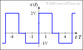
| − | We consider in this exercise a periodic and simultaneously ergodic stochastic process $\{x_i(t)\}$, which is fully characterized by the presented pattern function $x(t)$ | + | We consider in this exercise a periodic and simultaneously ergodic stochastic process $\{x_i(t)\}$, which is fully characterized by the presented pattern function $x(t)$. |
| − | Further pattern signals of the random process $\{x_i(t)\}$ are obtained by shifting by delays | + | Further pattern signals of the random process $\{x_i(t)\}$ are obtained by shifting by different delays $\tau_i$, where $\tau_i$ is assumed to be uniformly distributed between $0$ and the period $T_0$. |
| − | + | '''Hint:''' The exercise belongs to the chapter [[Theory_of_Stochastic_Signals/Auto-Correlation_Function|Auto-Correlation Function]]. | |
| − | |||
| − | |||
| − | |||
| − | |||
| − | Hint: | ||
| − | |||
| Line 22: | Line 16: | ||
<quiz display=simple> | <quiz display=simple> | ||
| − | {Determine the period duration $T_0$ normalized to the period duration $T$ defined in the sketch. | + | {Determine the period duration $T_0$ normalized to the period duration $T$ defined in the sketch. |
|type="{}"} | |type="{}"} | ||
$T_0/T \ = \ $ { 5 3% } | $T_0/T \ = \ $ { 5 3% } | ||
| − | {What is the size of the DC signal component | + | {What is the size of the DC signal component ⇒ linear mean $m_x$ of the described process $\{x_i(t)\}$? |
|type="{}"} | |type="{}"} | ||
$m_x \ = \ $ { 0.4 3% } $\ \rm V$ | $m_x \ = \ $ { 0.4 3% } $\ \rm V$ | ||
| − | {What is the process power (related to the resistor $1 \hspace{0.05cm} \rm \Omega$ )? | + | {What is the process power (related to the resistor $1 \hspace{0.05cm} \rm \Omega$ )? |
|type="{}"} | |type="{}"} | ||
$P_x \ = \ $ { 2 3% } $\ \rm V^2$ | $P_x \ = \ $ { 2 3% } $\ \rm V^2$ | ||
| − | {Calculate the | + | {Calculate the ACF values for $\tau = T$ and $\tau = 2T$. |
|type="{}"} | |type="{}"} | ||
$\varphi_x(\tau = T) \ = \ $ { 0.6 3% } $\ \rm V^2$ | $\varphi_x(\tau = T) \ = \ $ { 0.6 3% } $\ \rm V^2$ | ||
| Line 58: | Line 52: | ||
===Solution=== | ===Solution=== | ||
{{ML-Kopf}} | {{ML-Kopf}} | ||
| − | [[File:P_ID382__Sto_Z_4_9_d.png|right|frame|For ACF | + | [[File:P_ID382__Sto_Z_4_9_d.png|right|frame|For the ACF calculation]] |
| − | '''(1)''' The (normalized) period duration is $T_0/T \hspace{0.15cm}\underline{= 5}.$ | + | '''(1)''' The (normalized) period duration is $T_0/T \hspace{0.15cm}\underline{= 5}.$ |
| − | '''(2)''' Due to periodicity, the averaging | + | '''(2)''' Due to periodicity, the averaging over a periodic time $T_0$: |
:$$m_x = \frac{1}{T_0} \cdot \int_0^{T_0} x(t) \hspace{0.1cm}{\rm d} t = \frac{1}{5 T} \cdot (2\hspace{0.05cm}{\rm V} \cdot 2 T - 2\hspace{0.05cm}{\rm V} \cdot 2 T) \hspace{0.15cm}\underline{= \rm 0.4 \,V}.$$ | :$$m_x = \frac{1}{T_0} \cdot \int_0^{T_0} x(t) \hspace{0.1cm}{\rm d} t = \frac{1}{5 T} \cdot (2\hspace{0.05cm}{\rm V} \cdot 2 T - 2\hspace{0.05cm}{\rm V} \cdot 2 T) \hspace{0.15cm}\underline{= \rm 0.4 \,V}.$$ | ||
| − | '''(3)''' In analogy to the last | + | '''(3)''' In analogy to the last subtask, we obtain for the mean power: |
:$$P_x = \frac{2 T}{5 T} \cdot \big[(\rm 2V)^2 +(- \rm 1V)^2 \big]\hspace{0.15cm}\underline{ = \rm 2 \,V^2}.$$ | :$$P_x = \frac{2 T}{5 T} \cdot \big[(\rm 2V)^2 +(- \rm 1V)^2 \big]\hspace{0.15cm}\underline{ = \rm 2 \,V^2}.$$ | ||
'''(4)''' The accompanying graph shows in each case in the range from $0$ to $T_0 = 5T$. | '''(4)''' The accompanying graph shows in each case in the range from $0$ to $T_0 = 5T$. | ||
| − | *above the product $x(t) \cdot x(t+T)$, | + | :*above the product $x(t) \cdot x(t+T)$, |
| − | *down the product $x(t) \cdot x(t+2T)$. | + | :*down the product $x(t) \cdot x(t+2T)$. |
| − | Note that $x(t+T)$ means a shift of the signal $x(t)$ by $T$ to the left. | + | *Note that $x(t+T)$ means a shift of the signal $x(t)$ by $T$ to the left. |
| − | From these sketches follow the relations: | + | *From these sketches follow the relations: |
:$$\varphi_x (T)= \rm {1}/{5 } \cdot (\rm 4V^2 + \rm 1V^2 - \rm 2V^2) \hspace{0.15cm}\underline{= \rm 0.6\, V^2},$$ | :$$\varphi_x (T)= \rm {1}/{5 } \cdot (\rm 4V^2 + \rm 1V^2 - \rm 2V^2) \hspace{0.15cm}\underline{= \rm 0.6\, V^2},$$ | ||
:$$\varphi_x ( 2 T)= \rm {1}/{5 } \cdot(-\rm 2V^2 \cdot 3) \hspace{0.15cm}\underline{= - \rm 1.2 \,V^2}.$$ | :$$\varphi_x ( 2 T)= \rm {1}/{5 } \cdot(-\rm 2V^2 \cdot 3) \hspace{0.15cm}\underline{= - \rm 1.2 \,V^2}.$$ | ||
| − | '''(5)''' An auto-correlation function is always even: $\varphi_x (-\tau)= \varphi_x (\tau)$ | + | [[File:P_ID383__Sto_Z_4_9_e.png|right|frame|Wanted auto-correlation function]] |
| − | *In addition, for periodic processes, the ACF is also periodic with the same | + | '''(5)''' An auto-correlation function is always even: |
| − | + | :$$\varphi_x (-\tau)= \varphi_x (\tau).$$ | |
| + | *In addition, for periodic processes, the ACF is also periodic with the same period duration $T_0$ as the individual pattern functions. It follows that: | ||
:$$\varphi_x ( 0) = \varphi_x (5 T) = \varphi_x (10 T) = \ \text{...} \ = \it P_x = \rm 2 \,V^2,$$ | :$$\varphi_x ( 0) = \varphi_x (5 T) = \varphi_x (10 T) = \ \text{...} \ = \it P_x = \rm 2 \,V^2,$$ | ||
| Line 90: | Line 85: | ||
:$$\varphi_x (4 T) = \varphi_x (-4 T) =\varphi_x ( T) = \ \text{...} \ \hspace{0.15cm}\underline{= \rm 0.6 \,V^2}.$$ | :$$\varphi_x (4 T) = \varphi_x (-4 T) =\varphi_x ( T) = \ \text{...} \ \hspace{0.15cm}\underline{= \rm 0.6 \,V^2}.$$ | ||
| − | *The calculated ACF values can be connected by straight line sections, since integration | + | *The calculated ACF values can be connected by straight line sections, since integration over rectangular functions always yields linear subsections. |
| Line 96: | Line 91: | ||
'''(6)''' The five intervals $(0$ to $T)$, $(T$ to $2T)$, ... , $(4T$ to $5T)$ provide the contributions. | '''(6)''' The five intervals $(0$ to $T)$, $(T$ to $2T)$, ... , $(4T$ to $5T)$ provide the contributions. | ||
:$$(+1.3; -0.3; -1.2; -0.3; +1.3) \cdot \rm V^2.$$ | :$$(+1.3; -0.3; -1.2; -0.3; +1.3) \cdot \rm V^2.$$ | ||
| − | *This gives the expected value (linear mean): | + | *This gives the expected value (linear mean): |
:$${\rm E}\big[\varphi_x(\tau)\big] = 1/5 \cdot (1.3-0.3 -1.2 -0.3 +1.3]\hspace{0.15cm}\underline{= \rm 0.16 \,V^2}.$$ | :$${\rm E}\big[\varphi_x(\tau)\big] = 1/5 \cdot (1.3-0.3 -1.2 -0.3 +1.3]\hspace{0.15cm}\underline{= \rm 0.16 \,V^2}.$$ | ||
Latest revision as of 18:33, 19 March 2022
We consider in this exercise a periodic and simultaneously ergodic stochastic process $\{x_i(t)\}$, which is fully characterized by the presented pattern function $x(t)$.
Further pattern signals of the random process $\{x_i(t)\}$ are obtained by shifting by different delays $\tau_i$, where $\tau_i$ is assumed to be uniformly distributed between $0$ and the period $T_0$.
Hint: The exercise belongs to the chapter Auto-Correlation Function.
Questions
Solution
(1) The (normalized) period duration is $T_0/T \hspace{0.15cm}\underline{= 5}.$
(2) Due to periodicity, the averaging over a periodic time $T_0$:
- $$m_x = \frac{1}{T_0} \cdot \int_0^{T_0} x(t) \hspace{0.1cm}{\rm d} t = \frac{1}{5 T} \cdot (2\hspace{0.05cm}{\rm V} \cdot 2 T - 2\hspace{0.05cm}{\rm V} \cdot 2 T) \hspace{0.15cm}\underline{= \rm 0.4 \,V}.$$
(3) In analogy to the last subtask, we obtain for the mean power:
- $$P_x = \frac{2 T}{5 T} \cdot \big[(\rm 2V)^2 +(- \rm 1V)^2 \big]\hspace{0.15cm}\underline{ = \rm 2 \,V^2}.$$
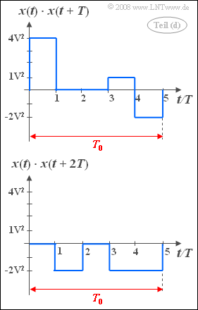
(4) The accompanying graph shows in each case in the range from $0$ to $T_0 = 5T$.
- above the product $x(t) \cdot x(t+T)$,
- down the product $x(t) \cdot x(t+2T)$.
- Note that $x(t+T)$ means a shift of the signal $x(t)$ by $T$ to the left.
- From these sketches follow the relations:
- $$\varphi_x (T)= \rm {1}/{5 } \cdot (\rm 4V^2 + \rm 1V^2 - \rm 2V^2) \hspace{0.15cm}\underline{= \rm 0.6\, V^2},$$
- $$\varphi_x ( 2 T)= \rm {1}/{5 } \cdot(-\rm 2V^2 \cdot 3) \hspace{0.15cm}\underline{= - \rm 1.2 \,V^2}.$$
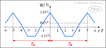
(5) An auto-correlation function is always even:
- $$\varphi_x (-\tau)= \varphi_x (\tau).$$
- In addition, for periodic processes, the ACF is also periodic with the same period duration $T_0$ as the individual pattern functions. It follows that:
- $$\varphi_x ( 0) = \varphi_x (5 T) = \varphi_x (10 T) = \ \text{...} \ = \it P_x = \rm 2 \,V^2,$$
- $$\varphi_x (3 T) = \varphi_x (-3 T) =\varphi_x (2 T) = \ \text{...} \ \hspace{0.15cm}\underline{= - \rm 1.2 \,V^2},$$
- $$\varphi_x (4 T) = \varphi_x (-4 T) =\varphi_x ( T) = \ \text{...} \ \hspace{0.15cm}\underline{= \rm 0.6 \,V^2}.$$
- The calculated ACF values can be connected by straight line sections, since integration over rectangular functions always yields linear subsections.
(6) The five intervals $(0$ to $T)$, $(T$ to $2T)$, ... , $(4T$ to $5T)$ provide the contributions.
- $$(+1.3; -0.3; -1.2; -0.3; +1.3) \cdot \rm V^2.$$
- This gives the expected value (linear mean):
- $${\rm E}\big[\varphi_x(\tau)\big] = 1/5 \cdot (1.3-0.3 -1.2 -0.3 +1.3]\hspace{0.15cm}\underline{= \rm 0.16 \,V^2}.$$
- This corresponds to the square of the mean $m_x$ ⇒ see subtask (2).


