Aufgaben:Exercise 4.14Z: Echo Detection

• Return to book

Echo measuring arrangement

To measure acoustic echoes in rooms  – for example caused by reflections at a wall –  the adjacent setup can be used:

• The noise generator produces a  "white noise in the relevant frequency range"  $x(t)$  with power density  $N_0 = 10^{-6} \hspace{0.08cm} \rm W/Hz$.
• This is bandlimited to  $B_x = 20 \hspace{0.08cm} \rm kHz$  and is given to a loudspeaker.
• The entire measurement setup is designed for the resistance value  $R = 50 \hspace{0.08cm} \rm \Omega$.

In the most general case,  the signal recorded by the microphone can be described as follows:

$$y(t) = \sum_{\mu = 1}^M \alpha_\mu \cdot x ( t - t_\mu ) .$$

Here the  $\alpha_\mu$  denote damping factors and  $t_\mu$  delay times.

Hints:

• The exercise belongs to the chapter  Cross-Correlation Function and Cross Power-Spectral Density.

• Use for numerical calculations the parameter values.

$$\alpha_1 = 0.5, \hspace{0.2cm}t_1 = 200 \,{\rm ms}, \hspace{0.2cm} \alpha_2 = 0.1, \hspace{0.2cm}t_2 = 250 \,{\rm ms}.$$

Questions

1

Apply the  $\rm ACF$  $\varphi_x(\tau)$  at the transmitter.  What means this converted to the resistor  $R = 50 \hspace{0.08cm} \rm \Omega$ ?  What is the rms value  $\sigma_x$ ?

$\sigma_x \ = \ $ $\ \rm V$

2

Calculate the cross-correlation function  $\rm (CCF)$   $\varphi_{xy}(\tau)$  between transmitted and received signal.
What values result for  $\tau = 0$,   $\tau = t_1 = 200 \hspace{0.08cm} \rm ms$   and   $\tau = t_2 = 250 \hspace{0.08cm} \rm ms$ ?

$\varphi_{xy}(\tau= 0) \ = \ $ $\ \rm V^2$

$\varphi_{xy}(\tau= t_1) \ = \ $ $\ \rm V^2$

$\varphi_{xy}(\tau= t_2) \ = \ $ $\ \rm V^2$

3

Calculate the cross power-spectral density   ${\it \Phi}_{xy}(f)$.  What value is obtained at frequency $f = 0$?

${\it \Phi}_{xy}(f =0)\ = \ $ $\ \cdot 10^{-6}\ \rm V^2\hspace{-0.1cm}/Hz$

4

Which of the following statements are true if you use the approximation  $\varphi_{xy}(\tau) \approx N_0/2 \cdot \delta(\tau)$  instead of the ACF calculated in  (1)?

	The noise is now  "true white"  – so it is not bandlimited.
	The noise power is reduced compared to subtask  (1).
	The cross-correlation function is the sum of weighted and shifted Dirac delta functions.
	The cross power-spectral density is calculated as in subtask  (3).

5

Calculate the  $\rm ACF$  $\varphi_y(\tau)$  using the approximation  $\varphi_{xy}(\tau) \approx N_0/2 \cdot \delta(\tau)$.   What weights result for   $\tau = 0$   and   $\tau = \Delta t = t_2 - t_1$?

$\varphi_{y}(\tau= 0) \ = \ $ $\ \cdot 10^{-6}\ \rm W\hspace{-0.1cm}/Hz$

$\varphi_{y}(\tau= \Delta t) \ = \ $ $\ \cdot 10^{-6}\ \rm W\hspace{-0.1cm}/Hz$

Solution

Solution

(1)  The two-sided power spectral density spectrum  ${\it \Phi}_{x}(f)$  is constantly equal  $N_0/2$ in the range  $\pm B_x$  .

• Whose Fourier transform is the ACF:

$$\varphi_x (\tau) = {N_0}/{2} \cdot 2 B_x \cdot {\rm si} (2 \pi B_x \tau) = 0.02 \hspace {0.08cm}{\rm W} \cdot {\rm si} (2 \pi B_x \tau).$$

• Converted from  $R = 50 \hspace{0.08cm} \rm \Omega$  to  $R = 1 \hspace{0.08cm} \rm \Omega$  thus one obtains  $($multiplication by  $R = 50 \hspace{0.08cm} \rm \Omega)$:

$$\varphi_x (\tau) = 0.02 \hspace {0.05cm}{\rm VA} \cdot 50 \hspace {0.05cm}{\rm V/A}\cdot {\rm si} (2 \pi B_x \tau)= 1 \hspace {0.05cm}{\rm V}^2 \cdot {\rm si} (2 \pi B_x \tau).$$

• The rms value is the square root of the ACF value at  $\tau = 0$:  

$$\sigma_x \hspace{0.15cm}\underline{= 1 \hspace {0.08cm}{\rm V}}.$$

(2)  For the cross correlation function (CCF), in the present case:

$$\varphi_{xy} (\tau) = \overline {x(t) \hspace{0.05cm}\cdot \hspace{0.05cm}y(t+\tau)} = \overline {x(t) \hspace{0.05cm}\cdot \hspace{0.05cm}\big [ \alpha_1 \cdot x(t- t_1+ \tau)\hspace{0.1cm}+\hspace{0.1cm} \alpha_2 \cdot x(t- t_2+ \tau)\big] } . $$

• After splitting the averaging on the two terms, we get:

$$\varphi_{xy} (\tau) = \alpha_1 \cdot \overline {x(t) \hspace{0.05cm}\cdot \hspace{0.05cm} x(t- t_1+ \tau)} \hspace{0.1cm}+\hspace{0.1cm} \alpha_2 \cdot \overline {x(t) \hspace{0.05cm}\cdot \hspace{0.05cm} x(t- t_2+ \tau)} .$$

• Using the ACF  $\varphi_x(\tau)$  can also be written herefor:

$$\varphi_{xy} (\tau) = \alpha_1 \cdot {\varphi_{x}(\tau- t_1)} \hspace{0.1cm}+\hspace{0.1cm} \alpha_2\cdot {\varphi_{x}(\tau- t_2)} = 1 \hspace {0.08cm}{\rm V}^2 \cdot \big[ \alpha_1 \cdot {\rm si} (2 \pi B_x (\tau - t_1)) + \alpha_2 \cdot {\rm si} (2 \pi B_x (\tau - t_2)) \big].$$

• The si function exhibits equidistant zero crossings at multiples of  $1/(2B_x) = 25 \hspace{0.08cm} µ \rm s$  respectively, related to the centers at  $t_1 = 200 \hspace{0.08cm} {\rm ms}$  and  $t_2 = 250 \hspace{0.08cm} {\rm ms}$.
• This results in the CCF values to:

$$\varphi_{xy} (\tau = 0) \hspace{0.15cm}\underline{= 0},\hspace{0.5cm}\varphi_{xy} (\tau = t_1)= \alpha_1 \cdot \varphi_{x} (\tau = 0) \hspace{0.15cm}\underline{= 0.5\,{\rm V}^2} ,\hspace{0.5cm} \varphi_{xy} (\tau = t_2)= \alpha_2 \cdot \varphi_{x} (\tau = 0) \hspace{0.15cm}\underline{= 0.1\,{\rm V}^2} .$$

(3)  The cross power spectral density is the Fourier transform of the CCF, just as the power spectral density spectrum (PSD) gives the Fourier transform of the ACF. For this holds:

$${\it \Phi}_{xy} (f) = \alpha_1 \cdot {\it \Phi}_{x} (f) \cdot {\rm e}^{-{\rm j}2 \pi f t_1} \hspace{0.15cm}+ \hspace{0.15cm}\alpha_2 \cdot {\it \Phi}_{x} (f) \cdot {\rm e}^{-{\rm j}2 \pi f t_2}. $$

• Outside the range  $|f| \le B_x$  the PSD  ${\it \Phi}_{x}(f)$  – and correspondingly the KPSD  ${\it \Phi}_{xy}(f)$ – is identically zero.
• In contrast, inside this interval holds  ${\it \Phi}_{x}(f) = N_0/2$. It follows in this range:

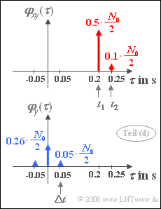
ACF and CCF in white noise

$${\it \Phi}_{xy} (f) = {N_0}/{2} \left( \alpha_1 \cdot {\rm e}^{-{\rm j}2 \pi f t_1} \hspace{0.15cm}+ \hspace{0.15cm}\alpha_2 \cdot {\rm e}^{-{\rm j}2 \pi f t_2} \right). $$

• It is evident that  ${\it \Phi}_{xy}(f)$  unlike  ${\it \Phi}_{x}(f)$  is a complex function.  For  $f = 0$  holds:

$${\it \Phi}_{xy} (f = 0) = {N_0}/{2} \left( \alpha_1 \hspace{0.15cm}+ \hspace{0.15cm}\alpha_2 \right) = 0.3 \cdot 10^{-6}\hspace{0.05cm}{\rm W/Hz} \hspace{0.15cm}\underline{= 15 \cdot 10^{-6}\hspace{0.07cm}{\rm V^2/Hz}} . $$

(4)  Correct are the proposed solutions 1 and 3:

• The Fourier transform of a dirac-shaped ACF leads to a constant PSD for all frequencies  $f$  that is, in fact, to "true white noise".
• This has an infinitely large power, and for the CCF can then be written according to the above graph:

$$\varphi_{xy} (\tau) = \alpha_1 \cdot { N_0}/{2} \cdot {\rm \delta}( \tau - t_1) \hspace {0.1cm}+ \hspace {0.1cm} \alpha_2 \cdot { N_0}/{2} \cdot { \rm \delta}( \tau - t_2) .$$

• In the frequency domain, indeed, no difference is detectable for  $|f| \le B_x$  compared to the subtask  (3)  .
• But since true white noise is now present, but here the cross power spectral density is not limited to this range.

(5)  For the ACF of the echoed signal,   $\varphi_{y} (\tau) = \overline {y(t) \hspace{0.05cm}\cdot \hspace{0.05cm}y(t+\tau)}$.

• This ACF $\varphi_{y} (\tau)$ can consequently be represented as the following sum:

$$\alpha_1^2 \cdot \overline {x(t - t_1) \cdot x(t - t_1+ \tau)} \hspace{0.03cm} + \hspace{0.03cm} \alpha_1\hspace{0.02cm}\alpha_2 \cdot \overline {x(t - t_1) \cdot x(t - t_2+ \tau)} + \hspace{0.05cm} \alpha_2\hspace{0.02cm}\alpha_1 \cdot \overline {x(t - t_2) \cdot x(t - t_1+ \tau)}\hspace{0.03cm} + \hspace{0.03cm} \alpha_2^2 \cdot \overline {x(t - t_2) \cdot x(t - t_2+ \tau)}. $$

• For the first and the last mean:

$$\overline {x(t - t_1) \hspace{0.05cm}\cdot \hspace{0.05cm}x(t - t_1+ \tau)} = \overline {x(t - t_2) \hspace{0.05cm}\cdot \hspace{0.05cm}x(t - t_2+ \tau)} = \overline {x(t ) \hspace{0.05cm}\cdot \hspace{0.05cm}x(t + \tau)} =\varphi_x(\tau).$$

• In contrast, for the second and third mean values, we obtain with  $\delta t = t_2 - t_1= 50 \ \rm ms$:

$$\overline {x(t - t_1) \hspace{0.05cm}\cdot \hspace{0.05cm}x(t - t_2+ \tau)} = \overline {x(t ) \hspace{0.05cm}\cdot \hspace{0.05cm}x(t + t_1- t_2+ \tau)} =\varphi_x(\tau - \Delta t),$$

$$\overline {x(t - t_2) \hspace{0.05cm}\cdot \hspace{0.05cm}x(t - t_1+ \tau)} = \overline {x(t ) \hspace{0.05cm}\cdot \hspace{0.05cm}x(t + t_2- t_1+ \tau)} =\varphi_x(\tau + \Delta t).$$

• Total, this again results in a symmetric ACF, as shown in the graph below:

$$\varphi_{y} (\tau) = {N_0}/{2} \cdot \left[ ( \alpha_1^2 \hspace{0.1cm} + \hspace{0.1cm} \alpha_2^2 ) \cdot {\rm \delta} (\tau) \hspace{0.1cm} + \hspace{0.1cm} \alpha_1 \cdot \alpha_2 \cdot {\rm \delta}(\tau - \delta t) \hspace{0.1cm} + \hspace{0.1cm} \alpha_1 \cdot \alpha_2 \cdot {\rm \delta}(\tau + \Delta t) \right].$$

$$\Rightarrow \hspace{0.3cm}\varphi_{y} (\tau = 0 ) \hspace{0.15cm}\underline{= 0.13 \cdot 10^{-6}\, {\rm W/Hz}}, \hspace{0.3cm}\varphi_{y} (\tau = \Delta t )\hspace{0.15cm}\underline{ = 0.025 \cdot 10^{-6}\, {\rm W/Hz}}.$$