Difference between revisions of "Aufgaben:Exercise 4.5: Mutual Information from 2D-PDF"
m (Guenter moved page Exercise 4.5: Mutual Information from 2D-WDF to Exercise 4.5: Mutual Information from 2D-PDF) |
|||
| Line 3: | Line 3: | ||
}} | }} | ||
| − | [[File:P_ID2886__Inf_A_4_5_neu.png|right|frame| | + | [[File:P_ID2886__Inf_A_4_5_neu.png|right|frame|Given joint PDF]] |
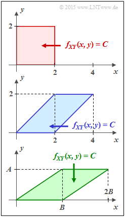
| − | + | Given here are the three different 2D regions $f_{XY}(x, y)$, which in the task are identified by their fill colors with | |
| − | * | + | * red joint PDF, |
| − | * | + | * blue joint PDF, und |
| − | * | + | * green joint PDF |
| − | + | respectively. Within each of the regions shown, let $f_{XY}(x, y) = C = \rm const.$ | |
| − | + | For example, the transinformation between the continuous-value random variables $X$ and $Y$ can be calculated as follows: | |
:$$I(X;Y) = h(X) + h(Y) - h(XY)\hspace{0.05cm}.$$ | :$$I(X;Y) = h(X) + h(Y) - h(XY)\hspace{0.05cm}.$$ | ||
| − | + | For the differential entropies used here, the following equations apply: | |
:$$h(X) = -\hspace{-0.7cm} \int\limits_{x \hspace{0.05cm}\in \hspace{0.05cm}{\rm supp}(f_X)} \hspace{-0.55cm} f_X(x) \cdot {\rm log} \hspace{0.1cm} \big[f_X(x)\big] \hspace{0.1cm}{\rm d}x | :$$h(X) = -\hspace{-0.7cm} \int\limits_{x \hspace{0.05cm}\in \hspace{0.05cm}{\rm supp}(f_X)} \hspace{-0.55cm} f_X(x) \cdot {\rm log} \hspace{0.1cm} \big[f_X(x)\big] \hspace{0.1cm}{\rm d}x | ||
\hspace{0.05cm},$$ | \hspace{0.05cm},$$ | ||
| Line 23: | Line 23: | ||
\hspace{-0.6cm} f_{XY}(x, y) \cdot {\rm log} \hspace{0.1cm} \big[ f_{XY}(x, y) \big] | \hspace{-0.6cm} f_{XY}(x, y) \cdot {\rm log} \hspace{0.1cm} \big[ f_{XY}(x, y) \big] | ||
\hspace{0.15cm}{\rm d}x\hspace{0.15cm}{\rm d}y\hspace{0.05cm}.$$ | \hspace{0.15cm}{\rm d}x\hspace{0.15cm}{\rm d}y\hspace{0.05cm}.$$ | ||
| − | * | + | *For the two marginal probability density functions, the following holds: |
:$$f_X(x) = \hspace{-0.5cm} \int\limits_{\hspace{-0.2cm}y \hspace{0.1cm}\in \hspace{0.1cm}{\rm supp} (f_{Y}\hspace{-0.08cm})} \hspace{-0.4cm} f_{XY}(x, y) | :$$f_X(x) = \hspace{-0.5cm} \int\limits_{\hspace{-0.2cm}y \hspace{0.1cm}\in \hspace{0.1cm}{\rm supp} (f_{Y}\hspace{-0.08cm})} \hspace{-0.4cm} f_{XY}(x, y) | ||
\hspace{0.15cm}{\rm d}y\hspace{0.05cm},$$ | \hspace{0.15cm}{\rm d}y\hspace{0.05cm},$$ | ||
| Line 35: | Line 35: | ||
| + | Hints: | ||
| + | *The exercise belongs to the chapter [[Information_Theory/AWGN–Kanalkapazität_bei_wertkontinuierlichem_Eingang|AWGN channel capacitance with continuous-value input]]. | ||
| − | + | *Let the following differential entropies also be given: | |
| − | + | :* If $X$ is triangularly distributed between $x_{\rm min}$ and $x_{\rm max}$, then: | |
| − | |||
| − | * | ||
| − | :* | ||
::$$h(X) = {\rm log} \hspace{0.1cm} [\hspace{0.05cm}\sqrt{ e} \cdot (x_{\rm max} - x_{\rm min})/2\hspace{0.05cm}]\hspace{0.05cm}.$$ | ::$$h(X) = {\rm log} \hspace{0.1cm} [\hspace{0.05cm}\sqrt{ e} \cdot (x_{\rm max} - x_{\rm min})/2\hspace{0.05cm}]\hspace{0.05cm}.$$ | ||
| − | :* | + | :* If $Y$ is equally distributed between $y_{\rm min}$ and $y_{\rm max}$, then holds: |
::$$h(Y) = {\rm log} \hspace{0.1cm} \big [\hspace{0.05cm}y_{\rm max} - y_{\rm min}\hspace{0.05cm}\big ]\hspace{0.05cm}.$$ | ::$$h(Y) = {\rm log} \hspace{0.1cm} \big [\hspace{0.05cm}y_{\rm max} - y_{\rm min}\hspace{0.05cm}\big ]\hspace{0.05cm}.$$ | ||
| − | * | + | *All results should be expressed in "bit". This is achieved with $\log$ ⇒ $\log_2$. |
| Line 50: | Line 49: | ||
| − | === | + | ===Questions=== |
<quiz display=simple> | <quiz display=simple> | ||
| − | { | + | {What is the mutual information of <u>the red joint PDF</u>? |
|type="{}"} | |type="{}"} | ||
$I(X; Y) \ = \ $ { 0. } $\ \rm bit$ | $I(X; Y) \ = \ $ { 0. } $\ \rm bit$ | ||
| − | { | + | {What is the mutual information of <u>the blue joint PDF</u>? |
|type="{}"} | |type="{}"} | ||
$I(X; Y) \ = \ $ { 0.721 3% } $\ \rm bit$ | $I(X; Y) \ = \ $ { 0.721 3% } $\ \rm bit$ | ||
| − | { | + | {What is the mutual information of <u>the green joint PDF</u>? |
|type="{}"} | |type="{}"} | ||
$I(X; Y) \ = \ $ { 0.721 3% } $\ \rm bit$ | $I(X; Y) \ = \ $ { 0.721 3% } $\ \rm bit$ | ||
| − | { | + | {What conditions must the random variables $X$ and $Y$ satisfy simultaneously for $I(X;Y) = 1/2 \cdot \log (\rm e)$ to hold in gener |
|type="[]"} | |type="[]"} | ||
| − | + | + | + The joint WDF $f_{XY}(x, y)$ results in a parallelogram. |
| − | + | + | + One of the random variables $(X$ or $Y)$ is uniformly distributed. |
| − | + | + | + The other random variable $(Y$ or $X)$ is triangularly distributed. |
| Line 77: | Line 76: | ||
</quiz> | </quiz> | ||
| − | === | + | ===Solution=== |
{{ML-Kopf}} | {{ML-Kopf}} | ||
| − | [[File:P_ID2887__Inf_A_4_5a.png|right|frame| | + | [[File:P_ID2887__Inf_A_4_5a.png|right|frame|„Red” PDFs]] |
| − | '''(1)''' | + | '''(1)''' For the rectangular joint PDF $f_{XY}(x, y)$ there are no statistical ties between $X$ and $Y$ ⇒ $\underline{I(X;Y) = 0}$. |
| − | + | Formally, this result can be proved with the following equation: | |
:$$I(X;Y) = h(X) \hspace{-0.05cm}+\hspace{-0.05cm} h(Y) \hspace{-0.05cm}- \hspace{-0.05cm}h(XY)\hspace{0.02cm}.$$ | :$$I(X;Y) = h(X) \hspace{-0.05cm}+\hspace{-0.05cm} h(Y) \hspace{-0.05cm}- \hspace{-0.05cm}h(XY)\hspace{0.02cm}.$$ | ||
| − | * | + | *The red area 2D-WDF $f_{XY}(x, y)$ is $F = 4$. Since $f_{XY}(x, y)$ is constant in this area and the volume under $f_{XY}(x, y)$ must be equal to $1$ , the height is $C = 1/F = 1/4$. |
| − | * | + | *From this follows for the differential joint entropy in "bit": |
:$$h(XY) \ = \ \hspace{0.1cm}-\hspace{0.2cm} \int \hspace{-0.9cm} \int\limits_{\hspace{-0.5cm}(x, y) \hspace{0.1cm}\in \hspace{0.1cm}{\rm supp} \hspace{0.03cm}(\hspace{-0.03cm}f_{XY}\hspace{-0.08cm})} | :$$h(XY) \ = \ \hspace{0.1cm}-\hspace{0.2cm} \int \hspace{-0.9cm} \int\limits_{\hspace{-0.5cm}(x, y) \hspace{0.1cm}\in \hspace{0.1cm}{\rm supp} \hspace{0.03cm}(\hspace{-0.03cm}f_{XY}\hspace{-0.08cm})} | ||
\hspace{-0.6cm} f_{XY}(x, y) \cdot {\rm log}_2 \hspace{0.1cm} [ f_{XY}(x, y) ] | \hspace{-0.6cm} f_{XY}(x, y) \cdot {\rm log}_2 \hspace{0.1cm} [ f_{XY}(x, y) ] | ||
| Line 92: | Line 91: | ||
\hspace{-0.6cm} f_{XY}(x, y) | \hspace{-0.6cm} f_{XY}(x, y) | ||
\hspace{0.15cm}{\rm d}x\hspace{0.15cm}{\rm d}y = 2 \,{\rm bit}\hspace{0.05cm}.$$ | \hspace{0.15cm}{\rm d}x\hspace{0.15cm}{\rm d}y = 2 \,{\rm bit}\hspace{0.05cm}.$$ | ||
| − | * | + | *It is considered that the double integral is equal to $1$ . The pseudo-unit "bit" corresponds to the <i>binary logarithm</i> ⇒ "log<sub>2</sub>". |
| + | |||
| + | Furthermore: | ||
| − | + | * The marginal probability density functions $f_{X}(x)$ and $f_{Y}(y)$ are rectangular ⇒ uniform distribution between $0$ and $2$: | |
| − | * | ||
:$$h(X) = h(Y) = {\rm log}_2 \hspace{0.1cm} (2) = 1 \,{\rm bit}\hspace{0.05cm}.$$ | :$$h(X) = h(Y) = {\rm log}_2 \hspace{0.1cm} (2) = 1 \,{\rm bit}\hspace{0.05cm}.$$ | ||
| − | * | + | * Substituting these results into the above equation, we obtain: |
:$$I(X;Y) = h(X) + h(Y) - h(XY) = 1 \,{\rm bit} + 1 \,{\rm bit} - 2 \,{\rm bit} = 0 \,{\rm (bit)} | :$$I(X;Y) = h(X) + h(Y) - h(XY) = 1 \,{\rm bit} + 1 \,{\rm bit} - 2 \,{\rm bit} = 0 \,{\rm (bit)} | ||
\hspace{0.05cm}.$$ | \hspace{0.05cm}.$$ | ||
| Line 104: | Line 104: | ||
| − | [[File:P_ID2888__Inf_A_4_5b_neu.png|right|frame| | + | [[File:P_ID2888__Inf_A_4_5b_neu.png|right|frame|„Blue” probability density functions]] |
| − | '''(2)''' | + | '''(2)''' Also for this parallelogram we get $F = 4, \ C = 1/4$ as well as $h(XY) = 2$ bit. |
| − | * | + | * Here, as in subtask '''(1)''' , the random variable $Y$ is uniformly distributed between $0$ and $2$ ⇒ $h(Y) = 1$ bit. |
| − | * | + | *In contrast, $X$ is triangularly distributed between $0$ and $4$ $($with maximum at $2)$. |
| − | * | + | *This results in the same differential entropy $h(Y)$ as for a symmetric triangular distribution in the range between $±2$ (see specification sheet): |
:$$h(X) = {\rm log}_2 \hspace{0.1cm} \big[\hspace{0.05cm}2 \cdot \sqrt{ e} \hspace{0.05cm}\big ] | :$$h(X) = {\rm log}_2 \hspace{0.1cm} \big[\hspace{0.05cm}2 \cdot \sqrt{ e} \hspace{0.05cm}\big ] | ||
= 1.721 \,{\rm bit}$$ | = 1.721 \,{\rm bit}$$ | ||
| Line 115: | Line 115: | ||
\hspace{0.05cm}.$$ | \hspace{0.05cm}.$$ | ||
<br clear=all> | <br clear=all> | ||
| − | [[File:P_ID2889__Inf_A_4_5c_neu.png|right|frame| | + | [[File:P_ID2889__Inf_A_4_5c_neu.png|right|frame|„Green” probability density functions]] |
| − | '''(3)''' | + | '''(3)''' The following properties are obtained for the green conditions: |
:$$F = A \cdot B \hspace{0.3cm} \Rightarrow \hspace{0.3cm} C = \frac{1}{A \cdot B} | :$$F = A \cdot B \hspace{0.3cm} \Rightarrow \hspace{0.3cm} C = \frac{1}{A \cdot B} | ||
\hspace{0.05cm}\hspace{0.3cm} | \hspace{0.05cm}\hspace{0.3cm} | ||
\Rightarrow \hspace{0.3cm} h(XY) = {\rm log}_2 \hspace{0.1cm} (A \cdot B) | \Rightarrow \hspace{0.3cm} h(XY) = {\rm log}_2 \hspace{0.1cm} (A \cdot B) | ||
\hspace{0.05cm}.$$ | \hspace{0.05cm}.$$ | ||
| − | * | + | *The random variable $Y$ is now uniformly distributed between $0$ and $A$ and the random variable $X$ is triangularly distributed between $0$ and $B$ : |
:$$h(X) \ = \ {\rm log}_2 \hspace{0.1cm} (B \cdot \sqrt{ e}) | :$$h(X) \ = \ {\rm log}_2 \hspace{0.1cm} (B \cdot \sqrt{ e}) | ||
\hspace{0.05cm},$$ $$ | \hspace{0.05cm},$$ $$ | ||
h(Y) \ = \ {\rm log}_2 \hspace{0.1cm} (A)\hspace{0.05cm}.$$ | h(Y) \ = \ {\rm log}_2 \hspace{0.1cm} (A)\hspace{0.05cm}.$$ | ||
| − | * | + | *Thus, for the mutual information between $X$ and $Y$: |
:$$I(X;Y) \ = {\rm log}_2 \hspace{0.1cm} (B \cdot \sqrt{ {\rm e}}) + {\rm log}_2 \hspace{0.1cm} (A) - {\rm log}_2 \hspace{0.1cm} (A \cdot B)$$ | :$$I(X;Y) \ = {\rm log}_2 \hspace{0.1cm} (B \cdot \sqrt{ {\rm e}}) + {\rm log}_2 \hspace{0.1cm} (A) - {\rm log}_2 \hspace{0.1cm} (A \cdot B)$$ | ||
:$$\Rightarrow \hspace{0.3cm} I(X;Y) = \ {\rm log}_2 \hspace{0.1cm} \frac{B \cdot \sqrt{ {\rm e}} \cdot A}{A \cdot B} = {\rm log}_2 \hspace{0.1cm} (\sqrt{ {\rm e}})\hspace{0.15cm}\underline{= 0.721\,{\rm bit}} | :$$\Rightarrow \hspace{0.3cm} I(X;Y) = \ {\rm log}_2 \hspace{0.1cm} \frac{B \cdot \sqrt{ {\rm e}} \cdot A}{A \cdot B} = {\rm log}_2 \hspace{0.1cm} (\sqrt{ {\rm e}})\hspace{0.15cm}\underline{= 0.721\,{\rm bit}} | ||
\hspace{0.05cm}.$$ | \hspace{0.05cm}.$$ | ||
| − | [[File: P_ID2890__Inf_A_4_5d.png |right|frame| | + | [[File: P_ID2890__Inf_A_4_5d.png |right|frame|Other examples of 2D PDF $f_{XY}(x, y)$]] |
| − | *$I(X;Y)$ | + | *$I(X;Y)$ thus independent of WDF parameters $A$ and $B$. |
| − | '''(4)''' <u> | + | '''(4)''' <u>All the above conditions</u> are required. |
| − | * | + | *However, the requirements '''(2)''' and '''(3)''' are not to be fulfilled for every parallelogram. The adjacent graphic shows two such constellations, where the random variable $X$ is in each case equally distributed between $0$ and $1$ . |
| − | * | + | * In the upper graph, the plotted points lie at a height ⇒ $f_{Y}(y)$ is triangularly distributed ⇒ $I(X;Y) = 0.721$ bit. |
| − | * | + | *The lower composite WDF has a different transinformation because the two points are not at the same height <br>⇒ die WDF $f_{Y}(y)$ has a trapezoidal shape here. |
| − | * | + | *Feeling-wise, I guess $I(X;Y) < 0.721$ bit, since the 2D area more closely approximates a rectangle. If you still feel like it, please check. |
{{ML-Fuß}} | {{ML-Fuß}} | ||
Revision as of 13:11, 29 September 2021
Given here are the three different 2D regions $f_{XY}(x, y)$, which in the task are identified by their fill colors with
- red joint PDF,
- blue joint PDF, und
- green joint PDF
respectively. Within each of the regions shown, let $f_{XY}(x, y) = C = \rm const.$
For example, the transinformation between the continuous-value random variables $X$ and $Y$ can be calculated as follows:
- $$I(X;Y) = h(X) + h(Y) - h(XY)\hspace{0.05cm}.$$
For the differential entropies used here, the following equations apply:
- $$h(X) = -\hspace{-0.7cm} \int\limits_{x \hspace{0.05cm}\in \hspace{0.05cm}{\rm supp}(f_X)} \hspace{-0.55cm} f_X(x) \cdot {\rm log} \hspace{0.1cm} \big[f_X(x)\big] \hspace{0.1cm}{\rm d}x \hspace{0.05cm},$$
- $$h(Y) = -\hspace{-0.7cm} \int\limits_{y \hspace{0.05cm}\in \hspace{0.05cm}{\rm supp}(f_Y)} \hspace{-0.55cm} f_Y(y) \cdot {\rm log} \hspace{0.1cm} \big[f_Y(y)\big] \hspace{0.1cm}{\rm d}y \hspace{0.05cm},$$
- $$h(XY) = \hspace{0.1cm}-\hspace{0.2cm} \int \hspace{-0.9cm} \int\limits_{\hspace{-0.5cm}(x, y) \hspace{0.1cm}\in \hspace{0.1cm}{\rm supp} (f_{XY}\hspace{-0.08cm})} \hspace{-0.6cm} f_{XY}(x, y) \cdot {\rm log} \hspace{0.1cm} \big[ f_{XY}(x, y) \big] \hspace{0.15cm}{\rm d}x\hspace{0.15cm}{\rm d}y\hspace{0.05cm}.$$
- For the two marginal probability density functions, the following holds:
- $$f_X(x) = \hspace{-0.5cm} \int\limits_{\hspace{-0.2cm}y \hspace{0.1cm}\in \hspace{0.1cm}{\rm supp} (f_{Y}\hspace{-0.08cm})} \hspace{-0.4cm} f_{XY}(x, y) \hspace{0.15cm}{\rm d}y\hspace{0.05cm},$$
- $$f_Y(y) = \hspace{-0.5cm} \int\limits_{\hspace{-0.2cm}x \hspace{0.1cm}\in \hspace{0.1cm}{\rm supp} (f_{X}\hspace{-0.08cm})} \hspace{-0.4cm} f_{XY}(x, y) \hspace{0.15cm}{\rm d}x\hspace{0.05cm}.$$
Hints:
- The exercise belongs to the chapter AWGN channel capacitance with continuous-value input.
- Let the following differential entropies also be given:
- If $X$ is triangularly distributed between $x_{\rm min}$ and $x_{\rm max}$, then:
- $$h(X) = {\rm log} \hspace{0.1cm} [\hspace{0.05cm}\sqrt{ e} \cdot (x_{\rm max} - x_{\rm min})/2\hspace{0.05cm}]\hspace{0.05cm}.$$
- If $Y$ is equally distributed between $y_{\rm min}$ and $y_{\rm max}$, then holds:
- $$h(Y) = {\rm log} \hspace{0.1cm} \big [\hspace{0.05cm}y_{\rm max} - y_{\rm min}\hspace{0.05cm}\big ]\hspace{0.05cm}.$$
- All results should be expressed in "bit". This is achieved with $\log$ ⇒ $\log_2$.
Questions
Solution
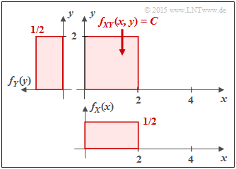
(1) For the rectangular joint PDF $f_{XY}(x, y)$ there are no statistical ties between $X$ and $Y$ ⇒ $\underline{I(X;Y) = 0}$.
Formally, this result can be proved with the following equation:
- $$I(X;Y) = h(X) \hspace{-0.05cm}+\hspace{-0.05cm} h(Y) \hspace{-0.05cm}- \hspace{-0.05cm}h(XY)\hspace{0.02cm}.$$
- The red area 2D-WDF $f_{XY}(x, y)$ is $F = 4$. Since $f_{XY}(x, y)$ is constant in this area and the volume under $f_{XY}(x, y)$ must be equal to $1$ , the height is $C = 1/F = 1/4$.
- From this follows for the differential joint entropy in "bit":
- $$h(XY) \ = \ \hspace{0.1cm}-\hspace{0.2cm} \int \hspace{-0.9cm} \int\limits_{\hspace{-0.5cm}(x, y) \hspace{0.1cm}\in \hspace{0.1cm}{\rm supp} \hspace{0.03cm}(\hspace{-0.03cm}f_{XY}\hspace{-0.08cm})} \hspace{-0.6cm} f_{XY}(x, y) \cdot {\rm log}_2 \hspace{0.1cm} [ f_{XY}(x, y) ] \hspace{0.15cm}{\rm d}x\hspace{0.15cm}{\rm d}y$$
- $$\Rightarrow \hspace{0.3cm} h(XY) \ = \ \ {\rm log}_2 \hspace{0.1cm} (4) \cdot \hspace{0.02cm} \int \hspace{-0.9cm} \int\limits_{\hspace{-0.5cm}(x, y) \hspace{0.1cm}\in \hspace{0.1cm}{\rm supp} \hspace{0.03cm}(\hspace{-0.03cm}f_{XY}\hspace{-0.08cm})} \hspace{-0.6cm} f_{XY}(x, y) \hspace{0.15cm}{\rm d}x\hspace{0.15cm}{\rm d}y = 2 \,{\rm bit}\hspace{0.05cm}.$$
- It is considered that the double integral is equal to $1$ . The pseudo-unit "bit" corresponds to the binary logarithm ⇒ "log2".
Furthermore:
- The marginal probability density functions $f_{X}(x)$ and $f_{Y}(y)$ are rectangular ⇒ uniform distribution between $0$ and $2$:
- $$h(X) = h(Y) = {\rm log}_2 \hspace{0.1cm} (2) = 1 \,{\rm bit}\hspace{0.05cm}.$$
- Substituting these results into the above equation, we obtain:
- $$I(X;Y) = h(X) + h(Y) - h(XY) = 1 \,{\rm bit} + 1 \,{\rm bit} - 2 \,{\rm bit} = 0 \,{\rm (bit)} \hspace{0.05cm}.$$
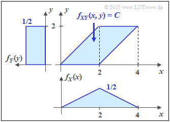
(2) Also for this parallelogram we get $F = 4, \ C = 1/4$ as well as $h(XY) = 2$ bit.
- Here, as in subtask (1) , the random variable $Y$ is uniformly distributed between $0$ and $2$ ⇒ $h(Y) = 1$ bit.
- In contrast, $X$ is triangularly distributed between $0$ and $4$ $($with maximum at $2)$.
- This results in the same differential entropy $h(Y)$ as for a symmetric triangular distribution in the range between $±2$ (see specification sheet):
- $$h(X) = {\rm log}_2 \hspace{0.1cm} \big[\hspace{0.05cm}2 \cdot \sqrt{ e} \hspace{0.05cm}\big ] = 1.721 \,{\rm bit}$$
- $$\Rightarrow \hspace{0.3cm} I(X;Y) = 1.721 \,{\rm bit} + 1 \,{\rm bit} - 2 \,{\rm bit}\hspace{0.05cm}\underline{ = 0.721 \,{\rm (bit)}} \hspace{0.05cm}.$$
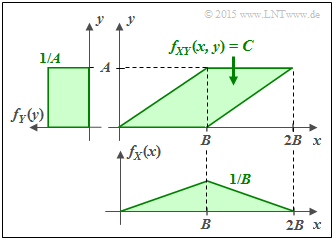
(3) The following properties are obtained for the green conditions:
- $$F = A \cdot B \hspace{0.3cm} \Rightarrow \hspace{0.3cm} C = \frac{1}{A \cdot B} \hspace{0.05cm}\hspace{0.3cm} \Rightarrow \hspace{0.3cm} h(XY) = {\rm log}_2 \hspace{0.1cm} (A \cdot B) \hspace{0.05cm}.$$
- The random variable $Y$ is now uniformly distributed between $0$ and $A$ and the random variable $X$ is triangularly distributed between $0$ and $B$ :
- $$h(X) \ = \ {\rm log}_2 \hspace{0.1cm} (B \cdot \sqrt{ e}) \hspace{0.05cm},$$ $$ h(Y) \ = \ {\rm log}_2 \hspace{0.1cm} (A)\hspace{0.05cm}.$$
- Thus, for the mutual information between $X$ and $Y$:
- $$I(X;Y) \ = {\rm log}_2 \hspace{0.1cm} (B \cdot \sqrt{ {\rm e}}) + {\rm log}_2 \hspace{0.1cm} (A) - {\rm log}_2 \hspace{0.1cm} (A \cdot B)$$
- $$\Rightarrow \hspace{0.3cm} I(X;Y) = \ {\rm log}_2 \hspace{0.1cm} \frac{B \cdot \sqrt{ {\rm e}} \cdot A}{A \cdot B} = {\rm log}_2 \hspace{0.1cm} (\sqrt{ {\rm e}})\hspace{0.15cm}\underline{= 0.721\,{\rm bit}} \hspace{0.05cm}.$$
- $I(X;Y)$ thus independent of WDF parameters $A$ and $B$.
(4) All the above conditions are required.
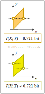
- However, the requirements (2) and (3) are not to be fulfilled for every parallelogram. The adjacent graphic shows two such constellations, where the random variable $X$ is in each case equally distributed between $0$ and $1$ .
- In the upper graph, the plotted points lie at a height ⇒ $f_{Y}(y)$ is triangularly distributed ⇒ $I(X;Y) = 0.721$ bit.
- The lower composite WDF has a different transinformation because the two points are not at the same height
⇒ die WDF $f_{Y}(y)$ has a trapezoidal shape here. - Feeling-wise, I guess $I(X;Y) < 0.721$ bit, since the 2D area more closely approximates a rectangle. If you still feel like it, please check.
