Difference between revisions of "Aufgaben:Exercise 4.7: Weighted Sum and Difference"
m (Text replacement - "Category:Aufgaben zu Stochastische Signaltheorie" to "Category:Theory of Stochastic Signals: Exercises") |
|||
| (7 intermediate revisions by 2 users not shown) | |||
| Line 1: | Line 1: | ||
| − | {{quiz-Header|Buchseite= | + | {{quiz-Header|Buchseite=Theory_of_Stochastic_Signals/Linear_Combinations_of_Random_Variables |
}} | }} | ||
| − | [[File:P_ID400__Sto_A_4_7.png|right|frame| | + | [[File:P_ID400__Sto_A_4_7.png|right|frame|Sum and difference of random variables]] |
| − | + | Let the random variables $u$ and $v$ be statistically independent of each other, each with mean $m$ and variance $\sigma^2$. | |
| − | * | + | *Both variables have equal probability density function $\rm (PDF)$ and cumulative distribution function $\rm (CDF)$. |
| − | * | + | *Nothing is known about the course of these functions for the time being. |
| − | + | Now two new random variables $x$ and $y$ are formed according to the following equations: | |
:$$x = A \cdot u + B \cdot v,$$ | :$$x = A \cdot u + B \cdot v,$$ | ||
:$$y= A \cdot u - B \cdot v.$$ | :$$y= A \cdot u - B \cdot v.$$ | ||
| − | + | Here, $A$ and $B$ denote (any) constant values. | |
| − | * | + | *For the subtasks '''(1)''' to '''(4)''' let $m= 0$, $\sigma = 1$, $A = 1$ and $B = 2$. |
| − | * | + | *In subtask '''(6)''' $u$ and $v$ are each uniformly distributed with $m= 1$ and $\sigma = 0.5$. For the constants, $A = B = 1$. |
| − | * | + | *For subtask '''(7)''' it is still valid $A = B = 1$. Here the random variables $u$ and $v$ are symmetrically two-point distributed on $\pm$1: |
:$${\rm Pr}(u=+1) = {\rm Pr}(u=-1) = {\rm Pr}(v=+1) = {\rm Pr}(v=-1) =0.5.$$ | :$${\rm Pr}(u=+1) = {\rm Pr}(u=-1) = {\rm Pr}(v=+1) = {\rm Pr}(v=-1) =0.5.$$ | ||
| Line 22: | Line 22: | ||
| − | + | Note: The exercise belongs to the chapter [[Theory_of_Stochastic_Signals/Linear_Combinations_of_Random_Variables|Linear Combinations of Random Variables]]. | |
| − | |||
| − | |||
| − | |||
| − | |||
| − | |||
| − | === | + | ===Questions=== |
<quiz display=simple> | <quiz display=simple> | ||
| − | { | + | {What is the mean and the standard deviation of $x$ for $A = 1$ and $B = 2$? |
|type="{}"} | |type="{}"} | ||
$m_x \ = \ $ { 0. } | $m_x \ = \ $ { 0. } | ||
| − | $\sigma_x \ = \ $ | + | $\sigma_x \ = \ $ { 2.236 3% } |
| − | { | + | {What is the mean and the standard deviation of $y$ for $A = 1$ and $B = 2$? |
|type="{}"} | |type="{}"} | ||
| − | $m_y \ = | + | $m_y \ = \ $ { 0. } |
| − | $\sigma_y \ = | + | $\sigma_y \ = \ $ { 2.236 3% } |
| − | { | + | {Calculate the covariance $\mu_{xy}$. What value results for $A = 1$ and $B = 2$? |
|type="{}"} | |type="{}"} | ||
| − | $\mu_{xy} \ = | + | $\mu_{xy} \ = \ $ { -3.09--2.91 } |
| − | { | + | {Calculate the correlation coefficient $\rho_{xy}$ as a function of the quotient $B/A$. What coefficient results for $A = 1$ and $B = 2$? |
|type="{}"} | |type="{}"} | ||
| − | $\rho_{xy}\ = | + | $\rho_{xy}\ = \ $ { -0.618--0.582 } |
| − | { | + | {Which of the following statements is always true? |
|type="[]"} | |type="[]"} | ||
| − | + | + | + For $B = 0$ the random variables $x$ and $y$ are strictly correlated. |
| − | - | + | - It holds $\rho_{xy}(-B/A) = -\rho_{xy}(B/A)$. |
| − | + | + | + In the limiting case $B/A \to \infty$ the random variables $x$ and $y$ are strictly correlated. |
| − | + | + | + For $A =B$ the random variables $x$ and $y$ are uncorrelated. |
| − | { | + | {Which statements are true if $A =B = 1$ holds and $x$ and $y$ are each Gaussian distributed with mean $m = 1$ and standard deviation $\sigma = 0.5$? |
|type="[]"} | |type="[]"} | ||
| − | + | + | + The random variables $x$ and $y$ are uncorrelated. |
| − | + | + | + The random variables $x$ and $y$ are statistically independent. |
| − | { | + | {Which statements are true if $x$ and $y$ are symmetrically two-point distributed and $A =B = 1$ holds? |
|type="[]"} | |type="[]"} | ||
| − | + | + | + The random variables $x$ and $y$ are uncorrelated. |
| − | - | + | - The random variables $x$ and $y$ are statistically independent. |
</quiz> | </quiz> | ||
| − | === | + | ===Solution=== |
{{ML-Kopf}} | {{ML-Kopf}} | ||
| − | '''(1)''' | + | '''(1)''' Since the random variables $u$ and $v$ are zero mean $(m = 0)$, the random variable $x$ is also zero mean: |
:$$m_x = (A +B) \cdot m \hspace{0.15cm}\underline{ =0}.$$ | :$$m_x = (A +B) \cdot m \hspace{0.15cm}\underline{ =0}.$$ | ||
| − | * | + | *For the variance and standard deviation: |
:$$\sigma_x^2 = (A^2 +B^2) \cdot \sigma^2 = 5; \hspace{0.5cm} \sigma_x = \sqrt{5}\hspace{0.15cm}\underline{ \approx 2.236}.$$ | :$$\sigma_x^2 = (A^2 +B^2) \cdot \sigma^2 = 5; \hspace{0.5cm} \sigma_x = \sqrt{5}\hspace{0.15cm}\underline{ \approx 2.236}.$$ | ||
| − | '''(2)''' | + | '''(2)''' Since $u$ and $v$ have the same standard deviation, so does $\sigma_y =\sigma_x \hspace{0.15cm}\underline{ \approx 2.236}$. |
| − | * | + | *Because $m=0$ also $m_y = m_x \hspace{0.15cm}\underline{ =0}$. |
| − | * | + | *For mean-valued random variable $u$ and $v$ on the other hand, for $m_y = (A -B) \cdot m$ adds up to a different value than for $m_x = (A +B) \cdot m$. |
| − | '''(3)''' | + | '''(3)''' We assume here in the sample solution the more general case $m \ne 0$. Then, for the common moment holds: |
:$$m_{xy} = {\rm E} \big[x \cdot y \big] = {\rm E} \big[(A \cdot u + B \cdot v) (A \cdot u - B \cdot v)\big] . $$ | :$$m_{xy} = {\rm E} \big[x \cdot y \big] = {\rm E} \big[(A \cdot u + B \cdot v) (A \cdot u - B \cdot v)\big] . $$ | ||
| − | * | + | *According to the general calculation rules for expected values, it follows: |
:$$m_{xy} = A^2 \cdot {\rm E} \big[u^2 \big] - B^2 \cdot {\rm E} \big[v^2 \big] = (A^2 - B^2)(m^2 + \sigma^2).$$ | :$$m_{xy} = A^2 \cdot {\rm E} \big[u^2 \big] - B^2 \cdot {\rm E} \big[v^2 \big] = (A^2 - B^2)(m^2 + \sigma^2).$$ | ||
| − | * | + | *This gives the covariance to |
| − | :$$\mu_{xy} = m_{xy} - m_{x} \cdot m_{y}= | + | :$$\mu_{xy} = m_{xy} - m_{x} \cdot m_{y}= (A^2 - B^2)(m^2 + \sigma^2) - (A + B)(A-B) \cdot m^2 = (A^2 - B^2) \cdot \sigma^2.$$ |
| − | * | + | *With $\sigma = 1$, $A = 1$ and $B = 2$ we get $\mu_{xy} \hspace{0.15cm}\underline{ =-3}$. Tthis is independent of the mean $m$ of the variables $u$ and $v$. |
| − | [[File:P_ID403__Sto_A_4_7_d_neu.png|right|frame| | + | [[File:P_ID403__Sto_A_4_7_d_neu.png|right|frame|correlation coefficient as a function of the quotient $B/A$]] |
| − | '''(4)''' | + | '''(4)''' The correlation coefficient is obtained as |
:$$\rho_{xy} =\frac{\mu_{xy}}{\sigma_x \cdot \sigma_y} = \frac{(A^2 - B^2) \cdot \sigma^2}{(A^2 +B^2) \cdot \sigma^2} | :$$\rho_{xy} =\frac{\mu_{xy}}{\sigma_x \cdot \sigma_y} = \frac{(A^2 - B^2) \cdot \sigma^2}{(A^2 +B^2) \cdot \sigma^2} | ||
\hspace{0.5 cm}\Rightarrow \hspace{0.5 cm}\rho_{xy} =\frac{1 - (B/A)^2} {1 +(B/A)^2}.$$ | \hspace{0.5 cm}\Rightarrow \hspace{0.5 cm}\rho_{xy} =\frac{1 - (B/A)^2} {1 +(B/A)^2}.$$ | ||
| − | * | + | *With $B/A = 2$ it follows $\rho_{xy} \hspace{0.15cm}\underline{ =-0.6}$. |
| − | '''(5)''' | + | '''(5)''' Correct are <u>statements 1, 3, and 4</u>: |
| − | * | + | *From $B= 0$ follows $\rho_{xy} = 1$ ("strict correlation"). It can be further seen that in this case $x = u$ and $y = u$ are identical random variables. |
| − | * | + | *The second statement is not true: For $A = 1$ and $B= -2$ also results $\rho_{xy} = -0.6$. |
| − | * | + | *So the sign of the quotient does not matter because in the equation calculated in subtask '''(4)'''' the quotient $B/A$ occurs only quadratically. |
| − | * | + | *If $B \gg A$, both $x$ and $y$ are determined almost exclusively by the random variable $v$ and it is $ y \approx -x$. This corresponds to the correlation coefficient $\rho_{xy} \approx -1$. |
| − | * | + | *In contrast, $B/A = 1$ always yields the correlation coefficient $\rho_{xy} = 0$ and thus the uncorrelatedness between $x$ and $y$. |
| − | '''(6)''' <u> | + | '''(6)''' <u>Both statements</u> are true: |
| − | * | + | *When $A=B$ ⇒ $x$ and $y$ are always uncorrelated $($for any PDF of the variables $u$ and $v)$. |
| − | * | + | *The new random variables $x$ and $y$ are therefore also distributed randomly. |
| − | * | + | *For Gaussian randomness, however, statistical independence follows from uncorrelatedness, and vice versa. |
| − | [[File:P_ID404__Sto_A_4_7_g.png|right|frame| | + | [[File:P_ID404__Sto_A_4_7_g.png|right|frame|Joint PDF and edge PDFs]] |
| − | '''(7)''' | + | '''(7)''' Here, only <u>statement 1</u> is true: |
| − | * | + | *The correlation coefficient results with $A=B= 1$ to $\rho_{xy} = 0$. That is: $x$ and $y$ are uncorrelated. |
| − | * | + | *But it can be seen from the sketched two-dimensional PDF that the condition of statistical independence no longer applies in the present case: |
| − | :$$f_{xy}(x, y) \ne f_{x}(x) \cdot | + | :$$f_{xy}(x, y) \ne f_{x}(x) \cdot f_{y}(y).$$ |
| Line 143: | Line 138: | ||
| − | [[Category:Theory of Stochastic Signals: Exercises|^4.3 | + | [[Category:Theory of Stochastic Signals: Exercises|^4.3 Linear Combinations^]] |
Latest revision as of 18:33, 25 February 2022
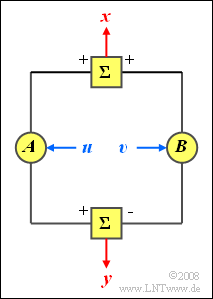
Let the random variables $u$ and $v$ be statistically independent of each other, each with mean $m$ and variance $\sigma^2$.
- Both variables have equal probability density function $\rm (PDF)$ and cumulative distribution function $\rm (CDF)$.
- Nothing is known about the course of these functions for the time being.
Now two new random variables $x$ and $y$ are formed according to the following equations:
- $$x = A \cdot u + B \cdot v,$$
- $$y= A \cdot u - B \cdot v.$$
Here, $A$ and $B$ denote (any) constant values.
- For the subtasks (1) to (4) let $m= 0$, $\sigma = 1$, $A = 1$ and $B = 2$.
- In subtask (6) $u$ and $v$ are each uniformly distributed with $m= 1$ and $\sigma = 0.5$. For the constants, $A = B = 1$.
- For subtask (7) it is still valid $A = B = 1$. Here the random variables $u$ and $v$ are symmetrically two-point distributed on $\pm$1:
- $${\rm Pr}(u=+1) = {\rm Pr}(u=-1) = {\rm Pr}(v=+1) = {\rm Pr}(v=-1) =0.5.$$
Note: The exercise belongs to the chapter Linear Combinations of Random Variables.
Questions
Solution
- $$m_x = (A +B) \cdot m \hspace{0.15cm}\underline{ =0}.$$
- For the variance and standard deviation:
- $$\sigma_x^2 = (A^2 +B^2) \cdot \sigma^2 = 5; \hspace{0.5cm} \sigma_x = \sqrt{5}\hspace{0.15cm}\underline{ \approx 2.236}.$$
(2) Since $u$ and $v$ have the same standard deviation, so does $\sigma_y =\sigma_x \hspace{0.15cm}\underline{ \approx 2.236}$.
- Because $m=0$ also $m_y = m_x \hspace{0.15cm}\underline{ =0}$.
- For mean-valued random variable $u$ and $v$ on the other hand, for $m_y = (A -B) \cdot m$ adds up to a different value than for $m_x = (A +B) \cdot m$.
(3) We assume here in the sample solution the more general case $m \ne 0$. Then, for the common moment holds:
- $$m_{xy} = {\rm E} \big[x \cdot y \big] = {\rm E} \big[(A \cdot u + B \cdot v) (A \cdot u - B \cdot v)\big] . $$
- According to the general calculation rules for expected values, it follows:
- $$m_{xy} = A^2 \cdot {\rm E} \big[u^2 \big] - B^2 \cdot {\rm E} \big[v^2 \big] = (A^2 - B^2)(m^2 + \sigma^2).$$
- This gives the covariance to
- $$\mu_{xy} = m_{xy} - m_{x} \cdot m_{y}= (A^2 - B^2)(m^2 + \sigma^2) - (A + B)(A-B) \cdot m^2 = (A^2 - B^2) \cdot \sigma^2.$$
- With $\sigma = 1$, $A = 1$ and $B = 2$ we get $\mu_{xy} \hspace{0.15cm}\underline{ =-3}$. Tthis is independent of the mean $m$ of the variables $u$ and $v$.
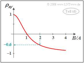
(4) The correlation coefficient is obtained as
- $$\rho_{xy} =\frac{\mu_{xy}}{\sigma_x \cdot \sigma_y} = \frac{(A^2 - B^2) \cdot \sigma^2}{(A^2 +B^2) \cdot \sigma^2} \hspace{0.5 cm}\Rightarrow \hspace{0.5 cm}\rho_{xy} =\frac{1 - (B/A)^2} {1 +(B/A)^2}.$$
- With $B/A = 2$ it follows $\rho_{xy} \hspace{0.15cm}\underline{ =-0.6}$.
(5) Correct are statements 1, 3, and 4:
- From $B= 0$ follows $\rho_{xy} = 1$ ("strict correlation"). It can be further seen that in this case $x = u$ and $y = u$ are identical random variables.
- The second statement is not true: For $A = 1$ and $B= -2$ also results $\rho_{xy} = -0.6$.
- So the sign of the quotient does not matter because in the equation calculated in subtask (4)' the quotient $B/A$ occurs only quadratically.
- If $B \gg A$, both $x$ and $y$ are determined almost exclusively by the random variable $v$ and it is $ y \approx -x$. This corresponds to the correlation coefficient $\rho_{xy} \approx -1$.
- In contrast, $B/A = 1$ always yields the correlation coefficient $\rho_{xy} = 0$ and thus the uncorrelatedness between $x$ and $y$.
(6) Both statements are true:
- When $A=B$ ⇒ $x$ and $y$ are always uncorrelated $($for any PDF of the variables $u$ and $v)$.
- The new random variables $x$ and $y$ are therefore also distributed randomly.
- For Gaussian randomness, however, statistical independence follows from uncorrelatedness, and vice versa.
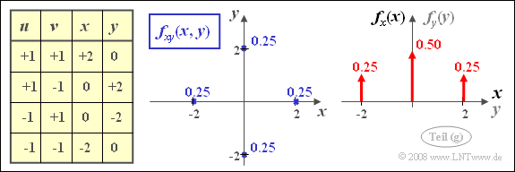
(7) Here, only statement 1 is true:
- The correlation coefficient results with $A=B= 1$ to $\rho_{xy} = 0$. That is: $x$ and $y$ are uncorrelated.
- But it can be seen from the sketched two-dimensional PDF that the condition of statistical independence no longer applies in the present case:
- $$f_{xy}(x, y) \ne f_{x}(x) \cdot f_{y}(y).$$


