Difference between revisions of "Aufgaben:Exercise 4.8: Diamond-shaped Joint PDF"
From LNTwww
m (Guenter moved page Exercise 4.8: Diamond shaped Joint PDF to Exercise 4.8: Diamond-shaped Joint PDF) |
|||
| Line 4: | Line 4: | ||
[[File:P_ID412__Sto_A_4_8.png|right|frame|Diamond shaped joint PDF]] | [[File:P_ID412__Sto_A_4_8.png|right|frame|Diamond shaped joint PDF]] | ||
| − | We consider a | + | We consider a two-dimensional random variable $(x,\hspace{0.08cm} y)$ whose components arise as linear combinations of two random variables $u$ and $v$: |
:$$x=2u-2v+1,$$ | :$$x=2u-2v+1,$$ | ||
:$$y=u+3v.$$ | :$$y=u+3v.$$ | ||
| − | Further, note: | + | Further, note: |
| − | *The two statistically independent random variables $u$ and $v$ are each | + | *The two statistically independent random variables $u$ and $v$ are each uniformly distributed between $0$ and $1$. |
| − | *In the figure you can see the | + | *In the figure you can see the joint PDF. Within the parallelogram drawn in blue holds: |
| − | :$$f_{xy}(x, y) = H = {\rm const.}$$ | + | :$$f_{xy}(x,\hspace{0.08cm} y) = H = {\rm const.}$$ |
| − | *Outside the parallelogram no values are possible: $f_{xy}(x, y) = 0$. | + | *Outside the parallelogram no values are possible: $f_{xy}(x,\hspace{0.08cm} y) = 0$. |
| − | + | Hints: | |
| − | |||
| − | |||
| − | |||
*The exercise belongs to the chapter [[Theory_of_Stochastic_Signals/Linear_Combinations_of_Random_Variables|Linear_Combinations of Random Variables]]. | *The exercise belongs to the chapter [[Theory_of_Stochastic_Signals/Linear_Combinations_of_Random_Variables|Linear_Combinations of Random Variables]]. | ||
| − | *Reference is also made to the page [[ | + | *Reference is also made to the page [[Theory_of_Stochastic_Signals/Two-Dimensional_Random_Variables#Regression_line|Regression line]]. |
| − | *We also refer here to the interactive applet [Applets:Korrelationskoeffizient_%26_Regressionsgerade|Correlation coefficient and regression line]] | + | *We also refer here to the interactive applet [[Applets:Korrelationskoeffizient_%26_Regressionsgerade|Correlation coefficient and regression line]] |
| − | *Assume - if possible - the given equations Use the information of the above sketch mainly only to check your results. | + | *Assume - if possible - the given equations. Use the information of the above sketch mainly only to check your results. |
Revision as of 19:09, 25 February 2022

Diamond shaped joint PDF
We consider a two-dimensional random variable $(x,\hspace{0.08cm} y)$ whose components arise as linear combinations of two random variables $u$ and $v$:
- $$x=2u-2v+1,$$
- $$y=u+3v.$$
Further, note:
- The two statistically independent random variables $u$ and $v$ are each uniformly distributed between $0$ and $1$.
- In the figure you can see the joint PDF. Within the parallelogram drawn in blue holds:
- $$f_{xy}(x,\hspace{0.08cm} y) = H = {\rm const.}$$
- Outside the parallelogram no values are possible: $f_{xy}(x,\hspace{0.08cm} y) = 0$.
Hints:
- The exercise belongs to the chapter Linear_Combinations of Random Variables.
- Reference is also made to the page Regression line.
- We also refer here to the interactive applet Correlation coefficient and regression line
- Assume - if possible - the given equations. Use the information of the above sketch mainly only to check your results.
Questions
Musterlösung
(1) Die Fläche des Parallelogramms kann aus zwei gleich großen Dreiecken zusammengesetzt werden.
- Die Fläche des Dreiecks $(1,0)\ (1,4)\ (-1,3)$ ergibt $0.5 · 4 · 2 = 4$.
- Die Gesamtfläche ist doppelt so groß: $F = 8$.
- Da das WDF–Volumen stets $1$ ist, gilt $H= 1/F\hspace{0.15cm}\underline{ = 0.125}$.
(2) Der minimale Wert von $x$ ergibt sich für $\underline{ u=0}$ und $\underline{ v=1}$.
- Daraus folgen aus obigen Gleichungen die Ergebnisse $x= -1$ und $y= +3$.
(3) Die im Theorieteil angegebene Gleichung gilt allgemein, also für jede beliebige WDF der beiden statistisch unabhängigen Größen $u$ und $v$,
- so lange diese gleiche Streuungen aufweisen $(\sigma_u = \sigma_v)$.
- Mit $A = 2$, $B = -2$, $D = 1$ und $E = 3$ erhält man:
- $$\rho_{xy } = \frac {\it A \cdot D + B \cdot E}{\sqrt{(\it A^{\rm 2}+\it B^{\rm 2})(\it D^{\rm 2}+\it E^{\rm 2})}} =\frac {2 \cdot 1 -2 \cdot 3}{\sqrt{(4 +4)(1+9)}} = \frac {-4}{\sqrt{80}} = \frac {-1}{\sqrt{5}}\hspace{0.15cm}\underline{ = -0.447}. $$
(4) Die Korrelationsgerade lautet allgemein:
- $$y=K(x)=\frac{\sigma_y}{\sigma_x}\cdot\rho_{xy}\cdot(x-m_x)+m_y.$$
- Aus den linearen Mittelwerten $m_u = m_v = 0.5$ und den in der Aufgabenstellung angegebenen Gleichungen erhält man $m_x = 1$ und $m_y = 2$.
- Die Varianzen von $u$ und $v$ betragen jeweils $\sigma_u^2 = \sigma_v^2 =1/12$. Daraus folgt:
- $$\sigma_x^2 = 4 \cdot \sigma_u^2 + 4 \cdot \sigma_v^2 = 2/3,$$
- $$\sigma_y^2 = \sigma_u^2 + 9\cdot \sigma_v^2 = 5/6.$$
- Setzt man diese Werte in die Gleichung der Korrelationsgeraden ein, so ergibt sich:
- $$y=K(x)=\frac{\sqrt{5/6}}{\sqrt{2/3}}\cdot (\frac{-1}{\sqrt{5}})\cdot(x-1)+2= - x/{2} + 2.5.$$
- Daraus folgt der Wert $y_0=K(x=0)\hspace{0.15cm}\underline{ = 2.5}$
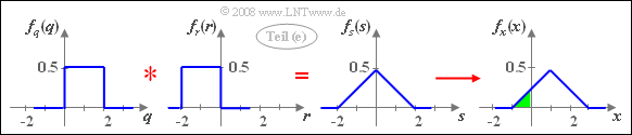
(5) Mit den Hilfsgrößen $q= 2u$, $r= -2v$ und $s= x-1$ gilt der Zusammenhang: $s= q+r$.
- Da $u$ und $v$ jeweils zwischen $0$ und $1$ gleichverteilt sind, besitzt $q$ eine Gleichverteilung im Bereich von $0$ bis $2$ und $r$ ist gleichverteilt zwischen $-2$ und $0$.
- Da zudem $q$ und $r$ nicht statistisch voneinander abhängen, gilt für die WDF der Summe:

Dreieckförmige WDF $f_x(x)$
- $$f_s(s) = f_q(q) \star f_r(r).$$
- Die Addition $x = s+1$ führt zu einer Verschiebung der Dreieck–WDF um $1$ nach rechts.
- Für die gesuchte Wahrscheinlichkeit (im folgenden Bild grün hinterlegt) gilt deshalb: ${\rm Pr}(x < 0)\hspace{0.15cm}\underline{ = 0.125}$.

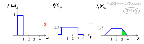
Trapezförmige WDF $f_y(y)$
(6) Analog zur Musterlösung für die Teilaufgabe (5) gilt mit $t = 3v$:
- $$f_y(y) = f_u(u) \star f_t(t).$$
- Die Faltung zwischen zwei verschieden breiten Rechtecken ergibt ein Trapez.
- Für die gesuchte Wahrscheinlichkeit erhält man ${\rm Pr}(y>3) =1/6\hspace{0.15cm}\underline{ \approx 0.167}$.
- Diese Wahrscheinlichkeit ist in der rechten Skizze grün hinterlegt.