Difference between revisions of "Aufgaben:Exercise 4.8: Diamond-shaped Joint PDF"
From LNTwww
(Die Seite wurde neu angelegt: „ {{quiz-Header|Buchseite=Stochastische Signaltheorie/Linearkombinationen von Zufallsgrößen }} right| :Wir betrachten eine 2…“) |
|||
| (22 intermediate revisions by 4 users not shown) | |||
| Line 1: | Line 1: | ||
| − | {{quiz-Header|Buchseite= | + | {{quiz-Header|Buchseite=Theory_of_Stochastic_Signals/Linear_Combinations_of_Random_Variables |
}} | }} | ||
| − | [[File:P_ID412__Sto_A_4_8.png|right|]] | + | [[File:P_ID412__Sto_A_4_8.png|right|frame|Diamond–shaped joint PDF]] |
| − | + | We consider a two-dimensional random variable $(x,\hspace{0.08cm} y)$ whose components arise as linear combinations of two random variables $u$ and $v$: | |
:$$x=2u-2v+1,$$ | :$$x=2u-2v+1,$$ | ||
:$$y=u+3v.$$ | :$$y=u+3v.$$ | ||
| − | : | + | Further, note: |
| + | *The two statistically independent random variables $u$ and $v$ are each uniformly distributed between $0$ and $1$. | ||
| + | *In the figure you can see the joint PDF. Within the parallelogram drawn in blue holds: | ||
| + | :$$f_{xy}(x,\hspace{0.08cm} y) = H = {\rm const.}$$ | ||
| + | *Outside the parallelogram no values are possible: $f_{xy}(x,\hspace{0.08cm} y) = 0$. | ||
| − | |||
| − | |||
| − | |||
| − | |||
| + | Hints: | ||
| + | *The exercise belongs to the chapter [[Theory_of_Stochastic_Signals/Linear_Combinations_of_Random_Variables|Linear Combinations of Random Variables]]. | ||
| + | *Reference is also made to the page [[Theory_of_Stochastic_Signals/Two-Dimensional_Random_Variables#Regression_line|Regression line]]. | ||
| + | *We also refer here to the interactive applet [[Applets:Korrelationskoeffizient_%26_Regressionsgerade|Correlation coefficient and regression line]] | ||
| + | *Assume - if possible - the given equations. Use the information of the above sketch mainly only to check your results. | ||
| + | |||
| − | === | + | |
| + | |||
| + | |||
| + | ===Questions=== | ||
<quiz display=simple> | <quiz display=simple> | ||
| − | { | + | {What is the height $H$ of the joint PDF within the parallelogram? |
|type="{}"} | |type="{}"} | ||
| − | $H$ | + | $H \ = \ $ { 0.125 3% } |
| − | { | + | {What values of $u$ and $v$ underlie the corner point $(-1, 3)$? |
|type="{}"} | |type="{}"} | ||
| − | $u$ | + | $u \ = \ $ { 0. } |
| − | $v$ | + | $v \ = \ $ { 1 3% } |
| − | { | + | {Calculate the correlation coefficient $\rho_{xy}$. |
|type="{}"} | |type="{}"} | ||
| − | $\rho_ | + | $\rho_{xy}\ = \ $ { -0.457--0.437 } |
| − | { | + | {What is the regression line $\rm (RL)$? At what point $y_0$ does it intersect the $y$–axis? |
|type="{}"} | |type="{}"} | ||
| − | $y_0$ | + | $y_0\ = \ $ { 2.5 3% } |
| − | { | + | {Calculate the marginal probability density function $f_x(x)$. What is the probability that the random variable $x$ is negative? |
|type="{}"} | |type="{}"} | ||
| − | $Pr(x < 0)$ | + | ${\rm Pr}(x < 0)\ = \ $ { 0.125 3% } |
| − | { | + | {Calculate the marginal probability density function $f_y(y)$. What is the probability that the random variablee $y >3$? |
|type="{}"} | |type="{}"} | ||
| − | $Pr(y > 3)$ | + | ${\rm Pr}(y > 3)\ = \ $ { 0.167 3% } |
</quiz> | </quiz> | ||
| − | === | + | ===Solution=== |
{{ML-Kopf}} | {{ML-Kopf}} | ||
| − | + | '''(1)''' The area of the parallelogram can be composed of two triangles of equal size. | |
| + | *The area of the triangle $(1,0)\ (1,4)\ (-1,3)$ gives $0.5 · 4 · 2 = 4$. | ||
| + | *The total area is double: $F = 8$. | ||
| + | *Since the PDF volume is always $1$ , then $H= 1/F\hspace{0.15cm}\underline{ = 0.125}$. | ||
| + | |||
| + | |||
| + | |||
| + | '''(2)''' The minimum value of $x$ is obtained for $\underline{ u=0}$ and $\underline{ v=1}$. | ||
| + | *From the above equations, the results $x= -1$ and $y= +3$ follow. | ||
| + | |||
| − | |||
| − | + | '''(3)''' The equation given in the theory section is valid in general, i.e., for any PDF of the two statistically independent variables $u$ and $v$, as long as they have equal standard deviations $(\sigma_u = \sigma_v)$. | |
| − | + | *With $A = 2$, $B = -2$, $D = 1$ and $E = 3$ we obtain: | |
:$$\rho_{xy } = \frac {\it A \cdot D + B \cdot E}{\sqrt{(\it A^{\rm 2}+\it B^{\rm 2})(\it D^{\rm 2}+\it E^{\rm 2})}} =\frac {2 \cdot 1 -2 \cdot 3}{\sqrt{(4 +4)(1+9)}} = \frac {-4}{\sqrt{80}} = \frac {-1}{\sqrt{5}}\hspace{0.15cm}\underline{ = -0.447}. $$ | :$$\rho_{xy } = \frac {\it A \cdot D + B \cdot E}{\sqrt{(\it A^{\rm 2}+\it B^{\rm 2})(\it D^{\rm 2}+\it E^{\rm 2})}} =\frac {2 \cdot 1 -2 \cdot 3}{\sqrt{(4 +4)(1+9)}} = \frac {-4}{\sqrt{80}} = \frac {-1}{\sqrt{5}}\hspace{0.15cm}\underline{ = -0.447}. $$ | ||
| − | |||
| − | |||
| − | + | '''(4)''' The regression line is generally: | |
| + | :$$y=\frac{\sigma_y}{\sigma_x}\cdot\rho_{xy}\cdot(x-m_x)+m_y.$$ | ||
| − | + | *From the linear means $m_u = m_v = 0.5$ and the equations given in the problem statement, we obtain $m_x = 1$ and $m_y = 2$. | |
| + | |||
| + | *The variances of $u$ and $v$ are respectively $\sigma_u^2 = \sigma_v^2 =1/12$. It follows: | ||
:$$\sigma_x^2 = 4 \cdot \sigma_u^2 + 4 \cdot \sigma_v^2 = 2/3,$$ | :$$\sigma_x^2 = 4 \cdot \sigma_u^2 + 4 \cdot \sigma_v^2 = 2/3,$$ | ||
:$$\sigma_y^2 = \sigma_u^2 + 9\cdot \sigma_v^2 = 5/6.$$ | :$$\sigma_y^2 = \sigma_u^2 + 9\cdot \sigma_v^2 = 5/6.$$ | ||
| − | + | *Substituting these values into the equation of the regression line, we get: | |
| − | :$$y | + | :$$y=\frac{\sqrt{5/6}}{\sqrt{2/3}}\cdot (\frac{-1}{\sqrt{5}})\cdot(x-1)+2= - x/{2} + 2.5.$$ |
| + | |||
| + | *From this follows with $x=0$ the value $y_0=\hspace{0.15cm}\underline{ = 2.5}$ | ||
| − | |||
| − | |||
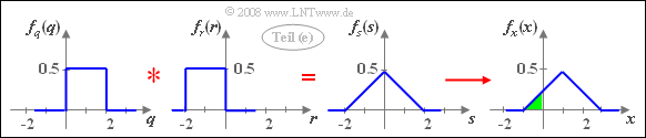
| − | : | + | '''(5)''' With the auxiliary quantities $q= 2u$, $r= -2v$ and $s= x-1$: $s= q+r$. |
| + | [[File:P_ID414__Sto_A_4_8_e.png|right|frame|Triangular PDF $f_x(x)$]] | ||
| + | *Since $u$ and $v$ are each uniformly distributed between $0$ and $1$, $q$ has a uniform distribution in the range from $0$ to $2$ and $r$ is uniformly distributed between $-2$ and $0$. | ||
| + | *In addition, since $q$ and $r$ are not statistically dependent on each other, the PDF of the sum is: | ||
:$$f_s(s) = f_q(q) \star f_r(r).$$ | :$$f_s(s) = f_q(q) \star f_r(r).$$ | ||
| + | *The addition $x = s+1$ leads to a shift of the triangular–PDF by $1$ to the right. | ||
| + | *For the sought probability (highlighted in green in the graphic) therefore holds: | ||
| + | :$${\rm Pr}(x < 0)\hspace{0.15cm}\underline{ = 0.125}.$$ | ||
| + | |||
| − | |||
| − | |||
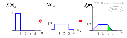
| − | : | + | [[File: P_ID415__Sto_A_4_8_f.png|right|frame|Trapezoidal PDF $f_y(y)$]] |
| + | '''(6)''' Analogous to the solution for the subtask '''(5)''' holds with $t = 3v$: | ||
:$$f_y(y) = f_u(u) \star f_t(t).$$ | :$$f_y(y) = f_u(u) \star f_t(t).$$ | ||
| − | + | *The convolution between two rectangles of different widths results in a trapezoid. For the probability we are looking for, we get: | |
| − | + | :$${\rm Pr}(y>3) =1/6\hspace{0.15cm}\underline{ \approx 0.167}.$$ | |
| + | *This probability is highlighted in green in the right sketch. | ||
| + | |||
| + | |||
{{ML-Fuß}} | {{ML-Fuß}} | ||
| − | [[Category: | + | [[Category:Theory of Stochastic Signals: Exercises|^4.3 Linear Combinations^]] |
Latest revision as of 15:07, 27 February 2022

Diamond–shaped joint PDF
We consider a two-dimensional random variable $(x,\hspace{0.08cm} y)$ whose components arise as linear combinations of two random variables $u$ and $v$:
- $$x=2u-2v+1,$$
- $$y=u+3v.$$
Further, note:
- The two statistically independent random variables $u$ and $v$ are each uniformly distributed between $0$ and $1$.
- In the figure you can see the joint PDF. Within the parallelogram drawn in blue holds:
- $$f_{xy}(x,\hspace{0.08cm} y) = H = {\rm const.}$$
- Outside the parallelogram no values are possible: $f_{xy}(x,\hspace{0.08cm} y) = 0$.
Hints:
- The exercise belongs to the chapter Linear Combinations of Random Variables.
- Reference is also made to the page Regression line.
- We also refer here to the interactive applet Correlation coefficient and regression line
- Assume - if possible - the given equations. Use the information of the above sketch mainly only to check your results.
Questions
Solution
(1) The area of the parallelogram can be composed of two triangles of equal size.
- The area of the triangle $(1,0)\ (1,4)\ (-1,3)$ gives $0.5 · 4 · 2 = 4$.
- The total area is double: $F = 8$.
- Since the PDF volume is always $1$ , then $H= 1/F\hspace{0.15cm}\underline{ = 0.125}$.
(2) The minimum value of $x$ is obtained for $\underline{ u=0}$ and $\underline{ v=1}$.
- From the above equations, the results $x= -1$ and $y= +3$ follow.
(3) The equation given in the theory section is valid in general, i.e., for any PDF of the two statistically independent variables $u$ and $v$, as long as they have equal standard deviations $(\sigma_u = \sigma_v)$.
- With $A = 2$, $B = -2$, $D = 1$ and $E = 3$ we obtain:
- $$\rho_{xy } = \frac {\it A \cdot D + B \cdot E}{\sqrt{(\it A^{\rm 2}+\it B^{\rm 2})(\it D^{\rm 2}+\it E^{\rm 2})}} =\frac {2 \cdot 1 -2 \cdot 3}{\sqrt{(4 +4)(1+9)}} = \frac {-4}{\sqrt{80}} = \frac {-1}{\sqrt{5}}\hspace{0.15cm}\underline{ = -0.447}. $$
(4) The regression line is generally:
- $$y=\frac{\sigma_y}{\sigma_x}\cdot\rho_{xy}\cdot(x-m_x)+m_y.$$
- From the linear means $m_u = m_v = 0.5$ and the equations given in the problem statement, we obtain $m_x = 1$ and $m_y = 2$.
- The variances of $u$ and $v$ are respectively $\sigma_u^2 = \sigma_v^2 =1/12$. It follows:
- $$\sigma_x^2 = 4 \cdot \sigma_u^2 + 4 \cdot \sigma_v^2 = 2/3,$$
- $$\sigma_y^2 = \sigma_u^2 + 9\cdot \sigma_v^2 = 5/6.$$
- Substituting these values into the equation of the regression line, we get:
- $$y=\frac{\sqrt{5/6}}{\sqrt{2/3}}\cdot (\frac{-1}{\sqrt{5}})\cdot(x-1)+2= - x/{2} + 2.5.$$
- From this follows with $x=0$ the value $y_0=\hspace{0.15cm}\underline{ = 2.5}$
(5) With the auxiliary quantities $q= 2u$, $r= -2v$ and $s= x-1$: $s= q+r$.

Triangular PDF $f_x(x)$
- Since $u$ and $v$ are each uniformly distributed between $0$ and $1$, $q$ has a uniform distribution in the range from $0$ to $2$ and $r$ is uniformly distributed between $-2$ and $0$.
- In addition, since $q$ and $r$ are not statistically dependent on each other, the PDF of the sum is:
- $$f_s(s) = f_q(q) \star f_r(r).$$
- The addition $x = s+1$ leads to a shift of the triangular–PDF by $1$ to the right.
- For the sought probability (highlighted in green in the graphic) therefore holds:
- $${\rm Pr}(x < 0)\hspace{0.15cm}\underline{ = 0.125}.$$

Trapezoidal PDF $f_y(y)$
(6) Analogous to the solution for the subtask (5) holds with $t = 3v$:
- $$f_y(y) = f_u(u) \star f_t(t).$$
- The convolution between two rectangles of different widths results in a trapezoid. For the probability we are looking for, we get:
- $${\rm Pr}(y>3) =1/6\hspace{0.15cm}\underline{ \approx 0.167}.$$
- This probability is highlighted in green in the right sketch.