Contents
Some characteristics of LDPC codes
The Low–density Parity–check Codes – in short LDPC codes – were invented as early as the early 1960s and date back to the dissertation [Gal63][1] by "Robert G. Gallager" .
However, the idea came several decades too early due to the processor technology of the time. Only three years after Berrou's invention of the turbo codes in 1993, however, David J. C. MacKay and "Radford M. Neal" recognized the huge potential of the LDPC codes if they were decoded iteratively symbol by symbol just like the turbo codes. They virtually reinvented the LDPC codes.
As can already be seen from the name component "parity–check", these codes are linear block codes according to the explanations in the "first main chapter" . Therefore, the same applies here:
- The code word results from the information word $\underline{u}$ (represented with $k$ binary symbols) and the "generator matrix" $\mathbf{G}$ of dimension $k × n$ to $\underline{x} = \underline{u} \cdot \mathbf{G}$ ⇒ code word length $n$.
- The parity-check equations result from the identity $\underline{x} \cdot \mathbf{H}^{\rm T} ≡ 0$, where $\mathbf{H}$ denotes the parity-check matrix. This consists of $m$ rows and $n$ columns. While in the first chapter basically $m = n -k$ was valid, for the LPDC codes we only require $m ≥ n -k$.
A serious difference between an LDPC code and a conventional block code as described in the first chapter is that the parity-check matrix $\mathbf{H}$ is sparsely populated with ones ("low-density').
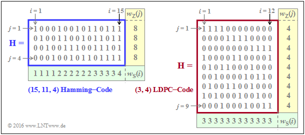
$\text{Example 1:}$ The graph shows parity-check matrices $\mathbf{H}$ for
- the Hamming code with code length $n = 15, \ m = 4$ ⇒ $k = 11$ information bits,
- the LDPC code from [Liv15][2] of length $n = 12$ and with $m = 9$ parity-check equations ⇒ $k ≥ 3$.
- In the left graph, the proportion of ones $32/60 \approx is 53.3\%$, whereas in the right graph the share of ones is lower with $36/108 = 33.3\%$ .
- For the LDPC codes (long length) relevant for practice, the share of ones is even significantly lower.
We now analyze the two parity-check matrices using the rate and Hamming weight:
- The rate of the Hamming code under consideration (left graph) is $R = k/n = 11/15 \approx 0.733$. The Hamming weight of each of the four rows is $w_{\rm Z}= 8$, while the Hamming weights $w_{\rm S}(i)$ of the columns vary between 1 and 4. For the columns index variable here: $1 ≤ i ≤ 15$.
- In the considered LDPC–code there are four ones in all rows ⇒ $w_{\rm Z} = 4$ and three ones in all columns ⇒ $w_{\rm S} = 3$. The code label $(w_{\rm Z}, \ w_{\rm S})$ LDPC code uses exactly these parameters. Note the different nomenclature to the "$(n, \ k, \ m)$ Hamming code".
- This is called a regular LDPC code, since all row weights $w_{\rm Z}(j)$ for $1 ≤ j ≤ m$ are constant equal $w_{\rm Z}$ and also all column weights $($with the indices $1 ≤ i ≤ n)$ are equal: $w_{\rm S}(i) = w_{\rm S} = {\rm const.}$ If this condition is not met, there is an irregular LDPC code.
$\text{Feature of LDPC codes}$ For the code rate, one can generally (if $k$ is not known) specify only one limit:
- $$R ≥ 1 - w_{\rm S}/w_{\rm Z}.$$
- The equal sign holds if all rows of $\mathbf{H}$ are linearly independent ⇒ $m = n \, – k$. Then the conventional equation is obtained:
- $$R = 1 - w_{\rm S}/w_{\rm Z} = 1 - m/n = k/n.$$
- In contrast, for the code rate of an irregular LDPC code and also for the $(15, 11, 4)$ Hamming code sketched on the left:
- $$R \ge 1 - \frac{ {\rm E}[w_{\rm S}]}{ {\rm E}[w_{\rm Z}]} \hspace{0.5cm}{\rm mit}\hspace{0.5cm} {\rm E}[w_{\rm S}] =\frac{1}{n} \cdot \sum_{i = 1}^{n}w_{\rm S}(i) \hspace{0.5cm}{\rm und}\hspace{0.5cm} {\rm E}[w_{\rm Z}] =\frac{1}{m} \cdot \sum_{j = 1}^{ m}w_{\rm Z}(j) \hspace{0.05cm}.$$
- Since in Hamming code the $m = n - k$ parity-check equations are linearly independent, the "$≥$"–sign can be replaced by the equal sign, which simultaneously means $R = k/n$ .
For more information on this topic, see "Exercise 4.11" and " Exercise 4.11Z".
Two-part LDPC graph representation - Tanner graph
All essential features of a LDPC ode are contained in the parity-check matrix $\mathbf{H} = (h_{j,\hspace{0.05cm}i})$ and can be represented by a so-called Tanner graph . It is a Bipartite Graph Representation. Before we examine and analyze exemplary Tanner graphs more exactly, first still some suitable description variables must be defined:
- The $n$ columns of the parity-check matrix $\mathbf{H}$ each represent one code word bit. Since each code word bit can be both an information bit and a check bit, the neutral name variable node (VN) has become accepted for this. The $i$th codeword bit is called $V_i$ and the set of all variable nodes (VNs) is $\{V_1, \text{...}\hspace{0.05cm} , \ V_i, \ \text{...}\hspace{0.05cm} , \ V_n\}$.
- The $m$ rows of $\mathbf{H}$ each describe a parity-check equation. We refer to such a parity-check equation as check node (CN) in the following. The set of all check nodes (CNs) is $\{C_1, \ \text{...}\hspace{0.05cm} , \ C_j, \ \text{...}\hspace{0.05cm} , \ C_m\}$, where $C_j$ denotes the parity-check equation of the $j$th row.
- In the Tanner–graph, the $n$ variable nodes $V_i$ as circles are represented as circles and the $m$ check nodes $C_j$ as squares. If the matrix element in row $j$ and column $i is \hspace{0.15cm} ⇒ \hspace{0.15cm} h_{j,\hspace{0.05cm}i} = 1$, there is an edge between the variable node $V_i$ and the check node $C_j$.
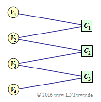
$\text{Example 2:}$ To clarify the above terms, an example Tanner graph is given on the right
- the Variable Nodes (short: VNs) $V_1$ to $V_4$, and
- the Check Nodes (short: CNs) $C_1$ to $C_3$.
However, the associated code has no practical meaning.
One can see from the graph:
- The code length is $n = 4$ and there are $m = 3$ parity-check equations. Thus the parity-check matrix $\mathbf{H}$ has dimension $3×4$.
- There are six edges in total. Thus six of the twelve elements $h_{j,\hspace{0.05cm}i}$ are of $\mathbf{H}$ ones.
- At each check node two lines arrive ⇒ The Hamming weights of all rows are equal: $w_{\rm S}(j) = 2 = w_{\rm S}$.
- From nodes $V_1$ and $V_4$ there is only one transition to a check node each, from $V_2$ nd $V_3$ however, there are two.
For this reason, it is an irregular code.
Accordingly, the parity-check matrix is:
- \[{ \boldsymbol{\rm H} } = \begin{pmatrix} 1 &1 &0 &0\\ 0 &1 &1 &0\\ 0 &0 &1 &1 \end{pmatrix}\hspace{0.05cm}.\]
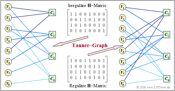
$\text{Example 3:}$ A more practical example now follows. In the "Exercise 4.11" two check matrices were analyzed:
- The encoder corresponding to the matrix $\mathbf{H}_1$ is systematic. The code parameters are $n = 8, \ k = 4$ and $m = 4$ ⇒ rate $1/2$. The code is irregular because the Hamming weights are not the same for all columns. In the graph, this "irregular $\mathbf{H}$ matrix" is given above.
- Bottom indicated is the "regular $\mathbf{H}$ matrix" corresponding to the matrix $\mathbf{H}_3$ in exercise 4.11. The rows are linear combinations of the upper matrix. For this non-systematic coder, with $w_{\rm S} = 2$ and $w_{\rm Z} = 4$ for the rate: $R \ge 1 - w_{\rm S}/w_{\rm Z} = 1/2$.
The graph shows the corresponding Tanner–s graphs:
- The left graph refers to the upper (irregular) matrix. The eight variable nodes (abbreviated VNs) $V_i$ are connected to the four check nodes (abbreviated CNs) $C_j$ if the element in row $j$ and column $i \hspace{0.15cm} ⇒ \hspace{0.15cm} h_{j,\hspace{0.05cm}i}$ is equal $1$ .
- This graph is not particularly well suited for "iterative symbol-wise decoding" . The VNs $V_5, \ \text{...}\hspace{0.05cm} , \ V_8$ are each associated with only one CN, which provides no information for decoding.
- In the right Tanner–s graph for the regular code, you can see that here from each variable node $V_i$ two edges come off and from each check node $C_j$ their four. This allows information to be gained during decoding in each iteration loop.
- It can also be seen that here, in the transition from the irregular to the equivalent regular code, the ones–share increases, in the example from $37.5\%$ to $50\%$. However, this statement cannot be generalized.
Iterative decoding of LDPC codes
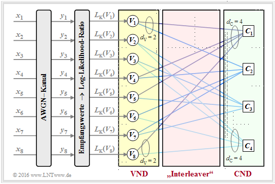
As an example of iterative LDPC–decoding, the so-called message–passing algorithm is now described. We illustrate this using the right-hand Tanner–graph in the $\text{"Example 3"}$ on the previous page and thus for the regular parity-check matrix given there.
$\text{Principle:}$ In the message–passing algorithm there is an alternating (or iterative) exchange of information between the (VNs) $V_1, \ \text{...}\hspace{0.05cm} , \ V_n$ and the check nodes (CNs) $C_1 , \ \text{...}\hspace{0.05cm} , \ C_m$.
For the example under consideration:
- There are $n = 8$ variable nodes and $m = 4$ check nodes . Since there is a regular LDPC–code, connecting lines go from each variable node $d_{\rm V} = 2$ to a check node and each check node is connected to $d_{\rm C} = 4$ variable nodes.
- The variable node degree $d_{\rm V}$ is equal to the Hamming weight of each column $(w_{\rm S})$ and for the check node degree holds: $d_{\rm C} = w_{\rm Z}$ (Hamming weight of each row).
- In the following description we also use the terms neighbors of a variable node ⇒ $N(V_i)$ and neighbors of a check node ⇒ $N(C_j)$, restricting ourselves here to implicit definitions:
- \[N(V_1) = \{ C_1, C_2\}\hspace{0.05cm}, \hspace{0.3cm}N(V_2) = \{ C_3, C_4\}\hspace{0.05cm}, \hspace{0.05cm}.\hspace{0.05cm}.\hspace{0.05cm}.\hspace{0.15cm},\hspace{0.3cm}N(V_8) = \{ C_1, C_4\}\hspace{0.05cm},\]
- \[N(C_1) = \{ V_1, V_4, V_5, V_8\}\hspace{0.05cm}, \hspace{0.05cm}.\hspace{0.05cm}.\hspace{0.05cm}.\hspace{0.15cm}\hspace{0.05cm}, \hspace{0.3cm}N(C_4) = \{ V_2, V_3, V_6, V_8\}\hspace{0.05cm}.\]
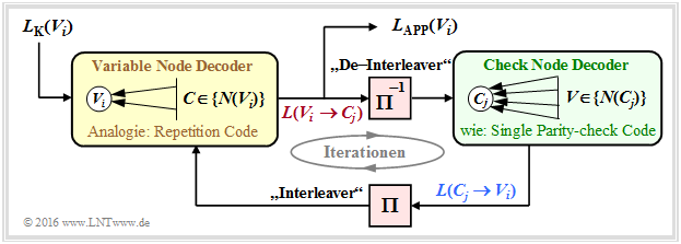
$\text{Example 4:}$ $\text{Example 4:}$ Die Skizze aus [Liv15][2] shows the exchange of information between the Variable Node $V_i$ and the Check Node $C_j$ – expressed by "Log–Likelihood Ratios" ($L$ values for short).
The exchange of information happens in two directions:
- $L(V_i → C_j)$: Extrinsic information from $V_i$–point of view, a priori–information from $C_j$–point of view.
- $L(C_j → V_i)$: Extrinsic information from $C_j$–point of view, a priori–information from $V_i$–point of view.
The description of the decoding algorithm continues:
Initialization: At the beginning of decoding, the variable nodes (VNs) receive no a priori–information from the check nodes (CNs), and it applies to $1 ≤ i ≤ n \text{:}$
- $$L(V_i → C_j) = L_{\rm K}(V_i).$$
As can be seen from the graph at the top of the page, these channel–$L$ values $L_{\rm K}(V_i)$ result from the received values $y_i$.
Check Node Decoder: Each node $C_j$ represents a parity-check equation. Thus $C_1$ represents the equation $V_1 + V_4 + V_5 + V_8 = 0$. One can see the connection to extrinsic information in the symbol-wise decoding of the Single Parity–check Code.
In analogy to the page "To calculate the extrinsic L–values" and to the "Exercise 4.4" thus applies to the extrinsic $L$–value of $C_j$ and at the same time to the a priori information concerning $V_i$:
- \[L(C_j \rightarrow V_i) = 2 \cdot {\rm tanh}^{-1}\left [ \prod\limits_{V \in N(C_j)\hspace{0.05cm},\hspace{0.1cm} V \ne V_i} \hspace{-0.35cm}{\rm tanh}\left [L(V \rightarrow C_j \right ] /2) \right ] \hspace{0.05cm}.\]
Variable Node Decoder: In contrast to the check node decoder (CND), the variable node decoder (VND) is related to the decoding of a repetition code because all check nodes connected to $V_i$ correspond to the same bit $C_j$ ⇒ this bit is repeated quasi $d_{\rm V}$ times.
In analogy to to the page "To calculate the extrinsic L values" applies to the extrinsic $L$ value of $V_i$ and at the same time to the a priori information concerning $C_j$:
- \[L(V_i \rightarrow C_j) = L_{\rm K}(V_i) + \hspace{-0.55cm} \sum\limits_{C \hspace{0.05cm}\in\hspace{0.05cm} N(V_i)\hspace{0.05cm},\hspace{0.1cm} C \hspace{0.05cm}\ne\hspace{0.05cm} C_j} \hspace{-0.55cm}L(C \rightarrow V_i) \hspace{0.05cm}.\]
The following diagram of the described decoding algorithm for LDPC–codes shows similarities with the procedure for "serial concatenated turbo codes".
- To establish a complete analogy between the LDPC and turbo decoding, an "interleaver " as well as an "deinterleaver " are also drawn here between the variable node decoder (VND) and the check node decoder (CND).
- Since these are not real system components, but only analogies, we have enclosed these terms in quotation marks.
Performance of regular LDPC codes
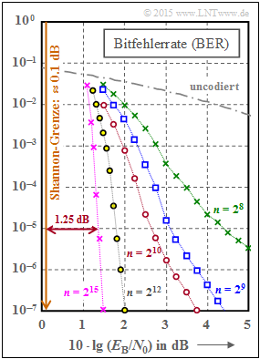
We now consider as in [Str14][3] five regular LDPC codes. The graph shows the bit error rate $\rm (BER)$ depending on the AWGN parameter $10 \cdot {\rm lg} \, E_{\rm B}/N_0$. The curve for uncoded transmission is also plotted for comparison.
These LDPC codes exhibit the following properties:
- The parity-check matrices $\mathbf{H}$ each have $n$ columns and $m = n/2$ linearly independent rows. In each row there are $w_{\rm Z} = 6$ ones and in each column $w_{\rm S} = 3$ ones.
- The share of ones is $w_{\rm Z}/n = w_{\rm S}/m$, so for large code word length $n$ the classification "low–density" is justified. For the red curve $(n = 2^{10})$ the share of ones is $0.6\%$.
- The rate of all codes is $R = 1 - w_{\rm S}/w_{\rm Z} = 1/2$. However, because of the linear independence of the matrix rows, $R = k/n$ with the information word length $k = n - m = n/2$ also holds.
From the graph you can see:
- The bit error rate is smaller the longer the code:
- For $10 \cdot {\rm lg} \, E_{\rm B}/N_0 = 2 \ \rm dB$ and $n = 2^8 = 256$ we get ${\rm BER} \approx 10^{-2}$.
- For $n = 2^{12} = 4096$ on the other hand, only ${\rm BER} \approx 2 \cdot 10^{-7}$.
- With $n = 2^{15} = 32768$ (violet curve) one needs $10 \cdot {\rm lg} \, E_{\rm B}/N_0 \approx 1.35 \ \rm dB$ for ${\rm BER} = 10^{-5}$.
- The distance from the Shannon limit $(0.18 \ \rm dB$ for $R = 1/2$ and BPSK$)$ is approximately $1.2 \ \rm dB$.
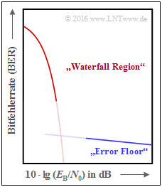
The curves for $n = 2^8$ to $n = 2^{10}$ also point to an effect we already noticed with the "turbo codes" :
- First, the BER curve drops steeply ⇒ "waterfall region".
- That is followed by a kink and a course with a significantly lower slope ⇒ "error floor".
- The qualitative lower graphic illustrates the effect, which of course does not start abruptly (transition not drawn).
An (LDPC) code is considered good whenever
- the BER curve drops steeply near the Shannon limit,
- the "error floor" is at very low BER values (for causes see next page, $\text{example 5)}$,
- the number of required iterations is manageable, and
- these properties are not reached only at no more practicable block lengths.
Performance of irregular LDPC codes
This chapter has dealt mainly with regular LDPC–codes, including in the $\rm BER$ diagram on the last page. The ignorance of irregular LDPC codes is only due to the brevity of this chapter, not their performance. On the contrary:
- Irregular LDPC codes are among the best channel codes ever.
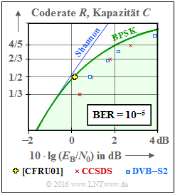
- The yellow cross in the graph is practically on the information-theoretical limit curve for binary input signals (green curve, labeled $\rm BPSK$).
- The codeword length of this irregular rate–$1/2$–code from [CFRU01][4] is $n = 2 \cdot 10^6$.
- From this it is already obvious that this code was not intended for practical use, but was even tuned for a record attempt.
The LDPC code construction always starts from the parity-check matrix $\mathbf{H}$ . For the just mentioned code this has the dimension $1 \cdot 10^6 × 2 \cdot 10^6$, thus contains $2 \cdot 10^{12}$ matrix elements.
$\text{Conclusion:}$ Filling the matrix randomly with (few) ones ⇒ "low–density" is called unstructured code design. This can lead to long codes with good performance, but sometimes also to the following problems:
- The complexity of the coder can increase, because despite modification of the parity-check matrix $\mathbf{H}$ it must be ensured that the generator matrix $\mathbf{G}$ is systematic.
- It requires a complex hardware–realization of the iterative decoder.
- It comes to an "error floor" by single ones in a column (or row) as well as by short loops ⇒ see following example.
$\text{Example 5:}$ The left part of the graph shows the Tanner graph for a regular LDPC code with the parity-check matrix $\mathbf{H}_1$ . Drawn in green is an example of the minimum girth. This parameter indicates the minimum number of edges one passes through before ending up at a check node $C_j$ again $($or from $V_i$ to $V_i)$. In the left example, the minimum edge length $6$, for example, results in the path $C_1 → V_1 → C_3 → V_5 → C_2 → V_2 → C_1$.
Swapping only two ones in the parity-check matrix ⇒ matrix $\mathbf{H}_2$, the LDPC code becomes irregular:
- The minimum loop length is now $4$, from $C_1 → V_4 → C_4 → V_6 → C_1$.
- A small girth leads to a pronounced "error floor" in the BER–process.
Einige Anwendungsgebiete für LDPC–Codes
Im nebenstehenden Schaubild sind im Vergleich zur AWGN–Kanalkapazität zwei Kommunikations–Standards eingetragen, die auf strukturierten (regulären) LDPC–Codes basieren.
Anzumerken ist, dass für die eingezeichneten standardisierten Codes die Bitfehlerrate ${\rm BER}=10^{-5}$ zugrunde liegt, während die Kapazitätskurven (entsprechend der Informationstheorie) für die Fehlerwahrscheinlichkeit "Null" gelten.
Rote Kreuze zeigen die LDPC–Codes nach CCSDS (Consultative Comittee for Space Data Systems), entwickelt für ferne Weltraummissionen:
- Diese Klasse stellt Codes der Rate $1/3$, $1/2$, $2/3$ und $4/5$ bereit.
- Alle Punkte liegen ca. $1 \ \rm dB$ rechts von der Kapazitätskurve für binären Eingang (grüne Kurve "BPSK").
Die blauen Rechtecke markieren die LDPC–Codes für DVB–T2/S2. Die Abkürzungen stehen für "Digital Video Broadcasting – Terrestrial" bzw. "Digital Video Broadcasting – Satellite", und die Kennzeichnung "$2$" macht deutlich, dass es sich jeweils um die zweite Generation (von 2005 bzw. 2009) handelt.
- Der Standard ist durch $22$ Prüfmatrizen definiert, die Raten von etwa $0.2$ bis zu $19/20$ zur Verfügung stellen.
- Je elf Varianten gelten für die Codelänge $64800$ Bit (Normal FECFRAME) bzw. $16200$ Bit (Short FECFRAME).
- Kombiniert mit "Modulationsverfahren hoher Ordnung" (8PSK, 16–ASK/PSK, ... ) zeichnen sich die Codes durch eine große spektrale Effizienz aus.
Die DVB–Codes gehören zu den Irregular Repeat Accumulate $\rm (IRA)$ Codes, die erstmals im Jahr 2000 in [JKE00][5] vorgestellt wurden.
Die Grafik zeigt die Grundstruktur des Coders.
- Der grün hinterlegte Teil – mit Repetition Code $\rm (RC)$, Interleaver, Single Parity–Code $\rm (SPC)$ sowie Akkumulator – entspricht exakt einem seriell–verketteten Turbocode ⇒ siehe "RA–Coder".
- Die Beschreibung des IRA–Codes basiert aber allein auf der Prüfmatrix $\mathbf{H}$, die sich durch den irregulären Repetition Code in eine für die Decodierung günstige Form bringen lässt.
- Als äußerer Code wird zudem ein hochratiger BCH–Code (von $\rm B$ose–$\rm C$haudhuri–$\rm H$ocquenghem) verwendet, der den Error Floor herabsetzen soll.
In der Grafik am Seitenanfang nicht eingetragen sind
- die LDPC–Codes für den Standard DVB Return Channel Terrestrial (RCS),
- die LDPC–Codes für den WiMax–Standard (IEEE 802.16), sowie
- die LDPC–Codes für das 10GBASE–T–Ethernet,
die gewisse Ähnlichkeiten mit den IRA–Codes aufweisen.
Aufgaben zum Kapitel
Aufgabe 4.11: Analyse von Prüfmatrizen
Zusatzaufgabe 4.11Z: Coderate aus der Prüfmatrix
Aufgabe 4.12: Regulärer/irregulärer Tanner–Graph
Aufgabe 4.13: Decodierung von LDPC–Codes
Quellenverzeichnis
- ↑ Gallager, R. G.: Low-density parity-check codes. MIT Press, Cambridge, MA, 1963.
- ↑ 2.0 2.1 Liva, G.: Channels Codes for Iterative Decoding. Lecture notes, Chair of Communications Engineering, TU Munich and DLR Oberpfaffenhofen, 2015. Cite error: Invalid
<ref>tag; name "Liv15" defined multiple times with different content - ↑ Strutz, T.: Low-density parity-check codes - An introduction. Lecture material. Hochschule für Telekommunikation, Leipzig, 2014. PDF document PDF document.
- ↑ Chung S.Y; Forney Jr., G.D.; Richardson, T.J.; Urbanke, R.: On the Design of Low-Density Parity- Check Codes within 0.0045 dB of the Shannon Limit. - In: IEEE Communications Letters, vol. 5, no. 2 (2001), pp. 58-60.
- ↑ Jin, H.; Khandekar, A.; McEliece, R.: Irregular Repeat–Accumulate Codes. Proc. of the 2nd Int. Symp. on Turbo Codes and Related Topics, Best, France, S. 1–8., Sept. 2000.
