Difference between revisions of "Mobile Communications/Distance Dependent Attenuation and Shading"
| Line 24: | Line 24: | ||
| − | == | + | == Physical description of the mobile communication channel == |
<br> | <br> | ||
[[File:EN_Mob_T1_1_S1.png|right|frame|Example for a mobile radio scenario|class=fit]] | [[File:EN_Mob_T1_1_S1.png|right|frame|Example for a mobile radio scenario|class=fit]] | ||
| Line 85: | Line 85: | ||
*For example, for [[Beispiele_von_Nachrichtensystemen/Allgemeine_Beschreibung_von_GSM|GSM/E–network]] $(f_{\rm S} = 1.8 \ \rm GHz$ ⇒ $\lambda \approx 17 \ \rm cm)$: $K_{\rm FR}(d = 1\ \rm km) = 1.6 \cdot 10^9$. The receiver at a distance of one kilometer does not receive even one billionth of the transmitting power.<br><br> | *For example, for [[Beispiele_von_Nachrichtensystemen/Allgemeine_Beschreibung_von_GSM|GSM/E–network]] $(f_{\rm S} = 1.8 \ \rm GHz$ ⇒ $\lambda \approx 17 \ \rm cm)$: $K_{\rm FR}(d = 1\ \rm km) = 1.6 \cdot 10^9$. The receiver at a distance of one kilometer does not receive even one billionth of the transmitting power.<br><br> | ||
| − | In the [[Aufgaben:Aufgabe_1.1Z:_Einfaches_Pfadverlustmodell| | + | In the [[Aufgaben:Aufgabe_1.1Z:_Einfaches_Pfadverlustmodell|Exercise 1.1Z]] the above Friis–equation is to be numerically evaluated and interpreted. Usually, the free space attenuation is set in relation to a suitable normalization distance to be defined $d_0$ ⇒ $K_{\rm FR}(d/d_0)$, where $d_0 = 1\ \rm m$ is often used.<br> |
== Common path loss model == | == Common path loss model == | ||
| Line 148: | Line 148: | ||
[[File:EN_Mob_T1_1_S5.png|right|frame|path loss without and with consideration of shading]] | [[File:EN_Mob_T1_1_S5.png|right|frame|path loss without and with consideration of shading]] | ||
<br> | <br> | ||
| + | |||
*The previous path loss models only take into account the distance-dependent signal attenuation according to the left graph and disregard topological factors such as the influence of shading. | *The previous path loss models only take into account the distance-dependent signal attenuation according to the left graph and disregard topological factors such as the influence of shading. | ||
| Line 165: | Line 166: | ||
*However, such channel changes are very slow due to shading. Often the conditions remain the same for several seconds and one speaks here of "Long Term Fading" in contrast to fast fading like [[Mobile_Kommunikation/Wahrscheinlichkeitsdichte_des_Rayleigh%E2%80%93Fadings#Allgemeine_Beschreibung_des_Mobilfunkkanals |Rayleigh–Fading]] and [[Mobile_Kommunikation/Nichtfrequenzselektives_Fading_mit_Direktkomponente#Kanalmodell_und_Rice.E2.80.93WDF| Rice–Fading.]]<br> | *However, such channel changes are very slow due to shading. Often the conditions remain the same for several seconds and one speaks here of "Long Term Fading" in contrast to fast fading like [[Mobile_Kommunikation/Wahrscheinlichkeitsdichte_des_Rayleigh%E2%80%93Fadings#Allgemeine_Beschreibung_des_Mobilfunkkanals |Rayleigh–Fading]] and [[Mobile_Kommunikation/Nichtfrequenzselektives_Fading_mit_Direktkomponente#Kanalmodell_und_Rice.E2.80.93WDF| Rice–Fading.]]<br> | ||
| − | == | + | == Lognormal channel model== |
<br> | <br> | ||
| − | [[File:EN_Mob_T1_1_S6.png|right|frame|Lognormal- | + | [[File:EN_Mob_T1_1_S6.png|right|frame|Lognormal-PDF ⇒ Shadowing loss]] |
| − | + | To account for the loss $V_{\rm S}$ by shadowing, the system design must be based on statistical models that have emerged from empirical studies. | |
| − | + | The best known is the '''Lognormal–channel model'', which uses a [[Stochastische_Signaltheorie/Gau%C3%9Fverteilte_Zufallsgr%C3%B6%C3%9Fe#Allgemeine_Beschreibung| Gaussian PDF]] for the random variable $V_{\rm S}$ : | |
::<math>f_{V_{\rm S}}(V_{\rm S}) = \frac {1}{ \sqrt{2 \pi }\cdot \sigma_{\rm S}} \cdot {\rm e }^{ - { (V_{\rm S}\hspace{0.05cm}- \hspace{0.05cm}m_{\rm S})^2}/(2 \hspace{0.05cm}\cdot \hspace{0.05cm}\sigma_{\rm S}^2) } \hspace{0.05cm}.</math> | ::<math>f_{V_{\rm S}}(V_{\rm S}) = \frac {1}{ \sqrt{2 \pi }\cdot \sigma_{\rm S}} \cdot {\rm e }^{ - { (V_{\rm S}\hspace{0.05cm}- \hspace{0.05cm}m_{\rm S})^2}/(2 \hspace{0.05cm}\cdot \hspace{0.05cm}\sigma_{\rm S}^2) } \hspace{0.05cm}.</math> | ||
| − | + | The name "lognormal" results from the fact that the dB–magnitude $V_{\rm S}$, which is derived from the linear power attenuation factor via the logarithm, is normally distributed (and thus Gaussian). <br> | |
| + | |||
| + | The lognormal–channel model is determined by two parameters: | ||
| + | *The mean value $m_{\rm S} = {\rm E}\big [V_{\rm S}\big ]$ gives the mean shadowing–loss. For rural areas it is usually calculated with $m_{\rm S} = 6 \ \rm dB$ for urban areas it is assumed $14 \ \rm dB$ ... $20 \ \rm dB$ off.<br> | ||
| − | + | *Also the standard deviation (or dispersion) $\sigma_{\rm S}$ is different for rural areas $(\approx 6 \ \rm dB)$ and for urban conditions $($between $8 \ \rm dB$ and $12 \ \rm dB)$ .<br><br> | |
| − | |||
| − | + | Note that $V_{\rm S}$ can also take negative values when using lognormal–fading (red background in the above graphic), which actually contradicts the idea of shading. In practice, however, this model has proven to be very good. | |
| − | |||
| − | + | The "gain by shading"; could be interpreted as follows: | |
| − | *In | + | *In urban canyons, reflections from buildings can cause more energy to arrive than would be expected after losing the path.<br> |
| − | * | + | *The path loss exponent $\gamma$ is always fixed, for example $\gamma = 3.76$ in urban areas. But there are positions in the city where $\gamma$ is smaller.<br> |
| − | * | + | *Such a simple model cannot reproduce all the details exactly, so one should not try to interpret all the model properties physically.<br><br> |
{{BlaueBox|TEXT= | {{BlaueBox|TEXT= | ||
| − | $\text{Fazit:}$ | + | $\text{Fazit:}$ It is useful to summarize the path loss portions in the following way: |
::<math>V_{\rm P} = V_{\rm 1} + V_{\rm 2}(t) \hspace{0.25cm}{\rm mit}\hspace{0.25cm} V_{\rm 1} = V_{\rm 0} + \gamma \cdot 10\,{\rm dB} \cdot {\rm lg} \hspace{0.1cm} (d/d_0)+ m_{\rm S}\hspace{0.05cm}.</math> | ::<math>V_{\rm P} = V_{\rm 1} + V_{\rm 2}(t) \hspace{0.25cm}{\rm mit}\hspace{0.25cm} V_{\rm 1} = V_{\rm 0} + \gamma \cdot 10\,{\rm dB} \cdot {\rm lg} \hspace{0.1cm} (d/d_0)+ m_{\rm S}\hspace{0.05cm}.</math> | ||
| − | + | The second term $V_{\rm 2}(t)$ now describes a lognormal–PDF with mean value zero: | |
::<math>f_{V_2}(V_2) = \frac {1}{ \sqrt{2 \pi }\cdot \sigma_{\rm S} } \cdot {\rm e }^{ - V_2 ^2/(2 \hspace{0.05cm}\cdot \hspace{0.05cm} \sigma_{\rm S}^2) }\hspace{0.05cm}.</math> | ::<math>f_{V_2}(V_2) = \frac {1}{ \sqrt{2 \pi }\cdot \sigma_{\rm S} } \cdot {\rm e }^{ - V_2 ^2/(2 \hspace{0.05cm}\cdot \hspace{0.05cm} \sigma_{\rm S}^2) }\hspace{0.05cm}.</math> | ||
| − | + | The distance dependency of $V_1$ does not play a major role and will not be further discussed here.}}<br> | |
| − | == | + | == Time domain model for lognormal fading== |
<br> | <br> | ||
| − | [[File:P ID2099 Mob T 1 1 S6b v2.png|right|frame| | + | [[File:P ID2099 Mob T 1 1 S6b v2.png|right|frame|ath loss model with lognormal fading]] |
| − | + | The figure shows a time domain model, with the help of which the path loss $V_{\rm P}$ can be simulated according to the above equation. Please note: | |
| − | * | + | *The input signal $s(t)$ possess the power $P_{\rm S}$. In logarithmic representation, the power is related to $1\ \rm mW$ and the pseudo unit "dBm" is added. |
| − | * | + | *The path loss $V_1$ is generated by multiplication with $k_1$ The output signal $r'(t)$ then has a power that is smaller by $V_1$ (in dB) : |
::<math>k_1 = 10^{-V_{\rm 1}/20} \hspace{0.1cm} \Rightarrow \hspace{0.1cm} | ::<math>k_1 = 10^{-V_{\rm 1}/20} \hspace{0.1cm} \Rightarrow \hspace{0.1cm} | ||
| Line 214: | Line 216: | ||
10 \cdot {\rm lg} \hspace{0.1cm} \frac{P_{\rm S} }{\rm 1\,mW} - V_1 | 10 \cdot {\rm lg} \hspace{0.1cm} \frac{P_{\rm S} }{\rm 1\,mW} - V_1 | ||
\hspace{0.05cm}.</math> | \hspace{0.05cm}.</math> | ||
| − | [[File:P ID2102 Mob T 1 1 S6c v3.png|right|frame| | + | [[File:P ID2102 Mob T 1 1 S6c v3.png|right|frame|Relation between Gauss $(V_2)$ und Lognormal $(z_2)$]] |
| − | * | + | *The (mean value-free) Lognormal–Fading is simulated by multiplication with the random variable $z_2(t)$ |
| − | * | + | *The PDF results from the Gaussian random quantity $V_2$ by a [[Stochastische_Signaltheorie/Exponentialverteilte_Zufallsgr%C3%B6%C3%9Fen#Transformation_von_Zufallsgr.C3.B6.C3.9Fen| nonlinear Transformation]] at the characteristic curve |
:$$z_2 = g(V_2) = 10^{-V_{\rm 2}/20}.$$ | :$$z_2 = g(V_2) = 10^{-V_{\rm 2}/20}.$$ | ||
| − | * | + | *For $z_2< 0$ this PDF is zero, and for $z_2\ge 0$ applies with the abbreviation $C = \rm ln(10)/20 dB$: |
:$$f_{z_{\rm 2}}(z_{\rm 2}) = \frac {{\rm e^{- {\rm ln}^2 (z_{\rm 2}) | :$$f_{z_{\rm 2}}(z_{\rm 2}) = \frac {{\rm e^{- {\rm ln}^2 (z_{\rm 2}) | ||
| Line 225: | Line 227: | ||
} } }{ \sqrt{2 \pi }\cdot C \cdot \sigma_{\rm S} \cdot z_2} \hspace{0.05cm}.$$ | } } }{ \sqrt{2 \pi }\cdot C \cdot \sigma_{\rm S} \cdot z_2} \hspace{0.05cm}.$$ | ||
| − | + | The graphic illustrates the transformation. You can see | |
| − | * | + | *the Gauss–PDF of $V_2$ (blue) with scatter $\sigma_{\rm S} = 6 \ \rm dB$, |
| − | * | + | *the negative logarithmic characteristic curve (green), and |
| − | * | + | *the asymmetric PDF (red) of the size to be multiplied $z_2(t)$. |
| − | + | We refer here to the [[Aufgaben:Aufgabe_1.2Z:_Nochmals_Lognormal–Fading|Exercise 1.2Z]]. | |
<br clear = all> | <br clear = all> | ||
| − | == | + | == Requirements for the following chapters == |
<br> | <br> | ||
| − | + | The average power of all signal components arriving at the receiver can be calculated using path loss and shading models. | |
| − | * | + | *The lognormal shadowing model takes into account slow changes of the reflectors due to the topology, with reception conditions changing only every five to ten meters in cities and every 30 to 100 meters in rural areas. |
| − | * | + | *In the following, the path loss and the influence of shadowing is not considered further, but on $1$ normalized.<br> |
| − | + | Paths can overlap constructively or destructively. The associated changes occur locally in the range of half the wavelength. In mobile radio, a few centimeters are enough to find completely different reception conditions. One speaks of '''Fast Fading'''. Such a channel is basically frequency– and time-dependent. | |
| − | + | For the rest of this first main chapter, frequency dependence is eliminated by assuming a single fixed frequency (see graph). | |
| − | [[File:P ID2100 Mob T 1 1 S7 v1.png|center|frame|Signale $s(t)$ | + | [[File:P ID2100 Mob T 1 1 S7 v1.png|center|frame|Signale $s(t)$ and $r(t)$ for the description of the mobile radio channel in bandpass–range (red) and in the equivalent low-pass range (blue); for the sketch $ϕ(t)\equiv 0$ ]] |
| − | + | The following conditions therefore apply with immediate effect: | |
| − | * | + | *The input signal of the mobile radio channel is a cosine oscillation with the amplitude $A = 1$ and the frequency $f_{\rm T}$. We refer to this harmonic oscillation as the „transmit signal” $s_{\rm BP}(t)$. This bandpass–signal is shown in red in the upper graphic.<br> |
| − | * | + | *The output signal $r_{\rm BP}(t)$ of the mobile radio channel – hereinafter „receive signal” called – may differ from $s_{\rm BP}(t)$ both in amplitude (envelope) and in phase ⇒ lower graph, red.<br> |
| − | * | + | *Furthermore, we mostly look at the mobile radio channel in the [[Signaldarstellung/%C3%84quivalentes_Tiefpass-Signal_und_zugeh%C3%B6rige_Spektralfunktion#Motivation| equivalent low-pass range.]] The "transmit signal" is then $s_{\rm TP}(t) = 1$ and thus real ⇒ blue horizontal in the upper graphic.<br> |
| − | * | + | *The LP–output signal $r_{\rm TP}(t)$ is generally complex, where the envelope is given by $a(t)$ and the phase $\phi(t)$ is noticeable by shifts in the zero crossings ⇒ blue envelope in the lower graph.<br><br> |
{{BlaueBox|TEXT= | {{BlaueBox|TEXT= | ||
| − | $\text{Fazit:}$ | + | $\text{Fazit:}$ For the '''physical (bandpass–)signal at the output of the mobile radio channel''' always applies in the following: |
::<math>r_{\rm BP}(t) = a(t) \cdot \cos \big [2\pi f_{\rm T} t + \phi(t)\big ]\hspace{0.3cm}\Rightarrow \hspace{0.3cm} a(t) = \vert r_{\rm BP}(t)\vert\hspace{0.05cm}, \hspace{0.2cm} \phi(t) = {\rm arc}\hspace{0.15cm} r_{\rm BP}(t)\hspace{0.05cm}.</math>}} | ::<math>r_{\rm BP}(t) = a(t) \cdot \cos \big [2\pi f_{\rm T} t + \phi(t)\big ]\hspace{0.3cm}\Rightarrow \hspace{0.3cm} a(t) = \vert r_{\rm BP}(t)\vert\hspace{0.05cm}, \hspace{0.2cm} \phi(t) = {\rm arc}\hspace{0.15cm} r_{\rm BP}(t)\hspace{0.05cm}.</math>}} | ||
| Line 266: | Line 268: | ||
| − | == | + | ==Exercises for the chapter == |
<br> | <br> | ||
[[Aufgaben:Exercise_1.1:_Dual_Slope_Loss_Model|Exercise 1.1: Dual Slope Loss Model]] | [[Aufgaben:Exercise_1.1:_Dual_Slope_Loss_Model|Exercise 1.1: Dual Slope Loss Model]] | ||
| − | [[Aufgaben:1.1Z_Einfaches_Pfadverlustmodell| | + | [[Aufgaben:1.1Z_Einfaches_Pfadverlustmodell|Exercise 1.1Z: Simple Path Loss Model]] |
| − | [[Aufgaben:1.2 Lognormal – Kanalmodell| | + | [[Aufgaben:1.2 Lognormal – Kanalmodell|Exercise 1.2: Lognormal - Channel Mode]] |
| − | [[Aufgaben:1.2Z_Nochmals_Lognormal–Fading| | + | [[Aufgaben:1.2Z_Nochmals_Lognormal–Fading|Exercise 1.2Z: Lognormal Fading Again]] |
==Quellenverzeichnis== | ==Quellenverzeichnis== | ||
Revision as of 04:24, 27 June 2020
Contents
- 1 # SYNOPSIS OF THE FIRST MAIN CHAPTER #
- 2 Physical description of the mobile communication channel
- 3 Free space propagation
- 4 Common path loss model
- 5 Other, more accurate path loss models
- 6 Additional loss due to shadowing
- 7 Lognormal channel model
- 8 Time domain model for lognormal fading
- 9 Requirements for the following chapters
- 10 Exercises for the chapter
- 11 Quellenverzeichnis
# SYNOPSIS OF THE FIRST MAIN CHAPTER #
The first main chapter deals with time-variant transmission channels, a property that is of great importance for mobile communication. The description is given throughout in the equivalent low-pass range.
It deals in detail with the following topics:
- the distance-dependent attenuation of a radio signal and various path loss models,
- the influence of shadowing , modelable through Lognormal-Fading
- the non-frequency selective Rayleigh fading for channels without "Line of Sight (LoS)",
- the consideration of the Doppler effect by the so-called Jakes spectrum
- the non-frequency selective Rice-Fading for channels with direct path (Line of Sight).
Physical description of the mobile communication channel
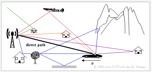
The figure shows a typical mobile radio scenario with a fixed base station and a mobile subscriber moving towards the base station at the speed $v$ .
In this representation, the radio signal reaches the mobile station via a direct path.
However, the antenna of the mobile subscriber also receives other signal components that reach the receiver in a detour, for example
- due to reflections on houses,
- a mountain range,
- a plane,
- the ionosphere,
- the ground.
This scenario can be used to explain important problems in mobile communications:
- Path Loss : This measures the attenuation of the electromagnetic wave, which depends to a large extent on the distance between transmitter and receiver.
- Shadowing : This describes a slow change in reception conditions due to the changing environment, for example when you pass a building or when you leave a wooded area.
- Multipath Propagation : If the signal reaches the receiver on several paths with differences in propagation time, constructive or destructive superimpositions up to complete extinction occur, depending on the signal frequency. For certain frequencies the topology is favorable, for others unfavorable. Therefore this effect is also called frequency selective fading
- Time Variance : The effect is caused by the movement of the transmitter and/or the receiver, because there is a different channel at each time. The transmission quality decreases rapidly if the direct path is shadowed by an obstacle. The received signal is then composed only of the partial signals arriving on detours, which are attenuated compared to the direct path due to scattering from trees and bushes and possibly refraction– and diffraction phenomena, and which add vectorially to the total signal.
- Doppler effect : Depending on whether (and also at what angle) the mobile station is moving towards or away from the transmitter, (slight) frequency shifts occur and thus statistical links within the received signal, which cause pulse interference .
In this chapter we will take a closer look at path loss and shadowing effects. The following chapters deal with time variance, also taking into account the Doppler effect. The second main chapter describes multipath propagation, which results in echoes in mobile radio.
Free space propagation
One speaks of "free space propagation" when there is a line of sight between the transmitter and the receiver positioned at a distance $d$ as in satellite communications or in space. The radio waves propagate in „empty space” unhindered spherically around the transmitting antenna, but are attenuated with increasing distance due to the law of conservation of energy.
Geometrically you can imagine that the radius $R$ of the sphere and thus also the spherical surface become larger and larger and at constant total energy the energy per unit area becomes proportional to $1/R^2$ smaller and smaller.
We assume an unmodulated oscillation of the frequency $f_{\rm S}$ or of the wavelength $\lambda= c/f_{\rm S}$ where $c = 3 \cdot 10^8\ \rm m/s$ indicates the speed of light , the signal power is $P_{\rm S}$.
Harald Friis gave an equation in 1944 for the reception power $P_{\rm E}(d)$ from the distance $d$ this equation, however, is only valid in a vacuum:
- \[P_{\rm E}(d) = \frac{P_{\rm S} \cdot G_{\rm S} \cdot G_{\rm E} \cdot \lambda^2}{16 \cdot \pi^2 \cdot d^2 \cdot V_{\rm zus}} = \frac{P_{\rm S} \cdot G_{\rm S} \cdot G_{\rm E} /V_{\rm zus}}{K_{\rm FR}(d)} \hspace{0.05cm}.\]
- $G_{\rm S}$ and $G_{\rm E}$ indicate the antenna gains of transmitter and receiver, respectively.
- $V_{\rm zus} > 1$ summarizes all additional losses independent of the wave propagation, e.g. through the antennas's cable feeds.
- The Free space attenuation $K_{\rm FR}(d)$ depends on the distance $d$ :
- \[K_{\rm FR}(d) = K_{\rm FR}(d_0) \cdot (d/d_0)^2 \hspace{0.2cm}{\rm mit} \hspace{0.2cm} K_{\rm FR}(d_0) = ({4 \pi d_0}/{\lambda} )^2 \hspace{0.05cm}.\]
Usually the free space attenuation is specified logarithmically with the pseudo unit „dB” Then the power loss due to free space attenuation ("V" stands for "Verlust" (loss) in dB):
- \[V_{\rm FR}(d) = 10 \cdot {\rm lg} \hspace{0.1cm} K_{\rm FR}(d) = V_{\rm 0} + 20\,\,{\rm dB} \cdot {\rm lg} \hspace{0.1cm} (d/d_0)\hspace{0.05cm},\hspace{0.5cm} V_{\rm 0} = V_{\rm FR}(d_0) = 20\,\,{\rm dB} \cdot {\rm lg} \hspace{0.2cm} ({4 \pi d_0}/{\lambda}) \hspace{0.05cm}.\]
It should be noted about this equation:
- The equation only applies in the far field of the antenna $(d > d_{\rm F})$. Here $d_{\rm F} = 2 D^2/\lambda$ the so-called Fraunhofer–Distance. For $D$ the largest physical dimension of the transmitting antenna must be used.
- The equation does not apply to $d \to 0$. This would result in the limit value $K_{\rm FR} \to 0$, and it would result independently from $P_{\rm S}$ always an infinite receiving power $P_{\rm E}(d \to 0)$.
- The free space attenuation $K_{\rm FR}(d)$ increases with increasing distance $d$ increases quadratically and also quadratically with increasing signal frequency $f_{\rm S}$, that is, with decreasing wavelength $\lambda$.
- For example, for GSM/E–network $(f_{\rm S} = 1.8 \ \rm GHz$ ⇒ $\lambda \approx 17 \ \rm cm)$: $K_{\rm FR}(d = 1\ \rm km) = 1.6 \cdot 10^9$. The receiver at a distance of one kilometer does not receive even one billionth of the transmitting power.
In the Exercise 1.1Z the above Friis–equation is to be numerically evaluated and interpreted. Usually, the free space attenuation is set in relation to a suitable normalization distance to be defined $d_0$ ⇒ $K_{\rm FR}(d/d_0)$, where $d_0 = 1\ \rm m$ is often used.
Common path loss model
In contrast to satellite and directional transmission links, in the case of land mobile radio, in addition to free-space attenuation, other disturbing effects which also contribute to a reduction in reception power must be taken into account, namely:
- Reflections: By superimposing the transmitted signal with a signal component reflected on the ground or on other large smooth surfaces, cancellations can occur which cause a decrease in the reception power up to the fourth power of the distance $d$ between transmitter and receiver. For more information, see [Zan05][1] and [PA95][2].
- Diffraction: This is when the signal is not reflected but deflected from its direction of propagation, for example at the edge of a building. A physical explanation can be found again in [Zan05][1].
- Dispersion: If the connection transmitter – receiver is interrupted by several objects with irregular surfaces (for example trees or bushes) the signal arrives at the receiver in the form of many scattered signals with slightly different propagation times. The size of the obstacle determines whether it is to be interpreted as a reflecting or as a scattering object.
The effects mentioned here are responsible for the fact that mobile radio can be operated without direct line of sight, and thus one of the bases for the economic success of mobile radio systems. Negatively, these effects are caused by a lower reception power, which must be taken into account by a larger exponent than $\gamma = 2$ . We then no longer speak of free space attenuation, but generally of "path attenuation factor":
- \[K_{\rm P}(d) = K_{\rm P}(d_0) \cdot (d/d_0)^\gamma \hspace{0.05cm}.\]
The corresponding dB–magnitude we call the path loss $(\rm lg$ is the logarithm to the base $10)$:
- \[V_{\rm P}(d) = V_{\rm 0} + \gamma \cdot 10\,{\rm dB} \cdot {\rm lg} \hspace{0.1cm} (d/d_0)\hspace{0.05cm},\hspace{0.5cm} V_{\rm 0} = V_{\rm P}(d_0) = \gamma \cdot 10\,{\rm dB} \cdot {\rm lg} \hspace{0.1cm} \frac{4 \cdot \pi \cdot d_0}{\lambda}\hspace{0.05cm}. \]
From these equations it can be seen that the free space attenuation $V_{\rm FR}(d)$ is a special case of $V_{\rm P}(d)$ with $\gamma = 2$ . In [Zan05][1] numerical values are given for the exponent $\gamma$ which were determined as mean values over a large number of measurements. Among other things
- in clear view (satellite, radio relay): $\gamma \approx 2$,
- in an urban setting: $\gamma = 2.7 \ \text{...} \ 3.5$,
- in a shaded urban setting: $\gamma = 3.0\ \text{...} \ 5.0$,
- Inside buildings without a line of sight: $\gamma = 4.0 \ \text{...} \ 6.0$.
Other, more accurate path loss models
The relatively simple path loss model shown on the last page is well suited for macro cells, but requires high base station antennas. It was used, for example, as a reference–scenario for the standardization of Long Term Evolution (LTE).
Of course, this very simple two–parameter model $(V_0, \ \gamma)$ cannot reproduce all use cases with sufficient accuracy. A large number of other models for power attenuation can be found in the literature, which are more precisely adapted to specific boundary conditions. (neighbourhood) and also take different cell sizes into account. Well-known are for example, siehe [Gol06][3]:
- the Okumura–Hata model,
- the path loss model according to COST 231,
- the Dual–Slope model.
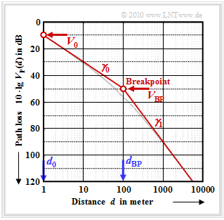
$\text{Example 1:}$ The Dual–Slope model is often used for simulations of micro cells in urban areas. The equation is the following, with the parameters $d_0 = 1\ \rm m$ und $d_{\rm BP}$ $($Breakpoint, beispielsweise $d_{\rm BP} = 100\ \rm m)$:
- \[V_{\rm P}(d) \hspace{-0.05cm} = \hspace{-0.05cm} V_{\rm 0} \hspace{-0.05cm}+\hspace{-0.05cm} \gamma_0 \hspace{-0.05cm}\cdot \hspace{-0.05cm} 10\,{\rm dB} \hspace{-0.05cm}\cdot \hspace{-0.05cm}{\rm lg} \hspace{0.01cm} \left ( {d}/{d_0} \right ) \hspace{-0.05cm}+ \hspace{-0.05cm}(\gamma_1 \hspace{-0.05cm}- \hspace{-0.05cm}\gamma_0) \hspace{-0.05cm}\cdot \hspace{-0.05cm}10\,{\rm dB} \hspace{-0.05cm}\cdot\hspace{-0.05cm} {\rm lg} \hspace{0.01cm} \left (1+ {d}/{d_{\rm BP} } \right )\hspace{0.05cm}.\]
The graph shows this curve for $V_{\rm 0} = 10 \ {\rm dB}$, $\gamma_0 = 2$ und $\gamma_1 = 4$ in the range from one meter to several kilometers (thin grey curve).
To simplify matters, the asymptotic approximation shown in red in the graph is used
- \[V_{\rm P}(d) = \left\{ \begin{array}{c} V_{\rm 0} + \gamma_0 \cdot 10\,{\rm dB} \cdot {\rm lg} \hspace{0.1cm} (d/d_0)\hspace{0.05cm},\\ V_{\rm BP} + \gamma_1 \cdot 10\,{\rm dB} \cdot {\rm lg} \hspace{0.1cm} (d/d_{\rm BP})\hspace{0.05cm}, \end{array} \right.\quad \begin{array}{*{1}c} {\rm f\ddot{u}r} \hspace{0.15cm}d < d_{\rm BP}\hspace{0.05cm}, \\ {\rm f\ddot{u}r} \hspace{0.15cm} d \ge d_{\rm BP}\hspace{0.05cm} \\ \end{array}\]
The value $V_{\rm BP} = 50 \ {\rm dB}$ is derived from the equation for the first section at the border $d = 100\ \rm m$ of the scope.
Note: In the Aufgabe 1.1 this model is still being examined in detail.
Additional loss due to shadowing
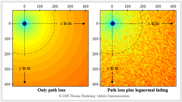
The disturbing influence of shading is explained with the help of a graphic, taken from the lecture manuscript [Hin08][4] :
- The previous path loss models only take into account the distance-dependent signal attenuation according to the left graph and disregard topological factors such as the influence of shading.
- In land mobile radio, shadowing (english: Shadowing) causes the signal level to vary even when moving at the same distance from the base station (on an arc of a circle) .
- This is shown in the right-hand graph, with darker areas indicating greater path loss. The difference between the left and right images is due to "Shadowing".
The effects of shadowing can be summarised as follows:
- For stationary transmitters and receivers, the shadowing is to be considered deterministic. It causes the path loss due to the shadowing to change by a constant value $V_{\rm S}$ (in dB):
- \[V_{\rm P}(d) = V_{\rm 0} + \gamma \cdot 10\,{\rm dB} \cdot {\rm lg} \hspace{0.1cm} (d/d_0)+ V_{\rm S}\hspace{0.05cm}. \]
- If the receiver (or the sender) moves, the shadowing–loss changes according to the coordinates and therefore also with time. This means: $V_{\rm S}$ ⇒ $V_{\rm S}(x, y)$ bzw. $V_{\rm S}$ ⇒ $V_{\rm S}(t)$.
- However, such channel changes are very slow due to shading. Often the conditions remain the same for several seconds and one speaks here of "Long Term Fading" in contrast to fast fading like Rayleigh–Fading and Rice–Fading.
Lognormal channel model
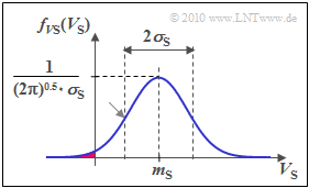
To account for the loss $V_{\rm S}$ by shadowing, the system design must be based on statistical models that have emerged from empirical studies.
The best known is the 'Lognormal–channel model, which uses a Gaussian PDF for the random variable $V_{\rm S}$ :
- \[f_{V_{\rm S}}(V_{\rm S}) = \frac {1}{ \sqrt{2 \pi }\cdot \sigma_{\rm S}} \cdot {\rm e }^{ - { (V_{\rm S}\hspace{0.05cm}- \hspace{0.05cm}m_{\rm S})^2}/(2 \hspace{0.05cm}\cdot \hspace{0.05cm}\sigma_{\rm S}^2) } \hspace{0.05cm}.\]
The name "lognormal" results from the fact that the dB–magnitude $V_{\rm S}$, which is derived from the linear power attenuation factor via the logarithm, is normally distributed (and thus Gaussian).
The lognormal–channel model is determined by two parameters:
- The mean value $m_{\rm S} = {\rm E}\big [V_{\rm S}\big ]$ gives the mean shadowing–loss. For rural areas it is usually calculated with $m_{\rm S} = 6 \ \rm dB$ for urban areas it is assumed $14 \ \rm dB$ ... $20 \ \rm dB$ off.
- Also the standard deviation (or dispersion) $\sigma_{\rm S}$ is different for rural areas $(\approx 6 \ \rm dB)$ and for urban conditions $($between $8 \ \rm dB$ and $12 \ \rm dB)$ .
Note that $V_{\rm S}$ can also take negative values when using lognormal–fading (red background in the above graphic), which actually contradicts the idea of shading. In practice, however, this model has proven to be very good.
The "gain by shading"; could be interpreted as follows:
- In urban canyons, reflections from buildings can cause more energy to arrive than would be expected after losing the path.
- The path loss exponent $\gamma$ is always fixed, for example $\gamma = 3.76$ in urban areas. But there are positions in the city where $\gamma$ is smaller.
- Such a simple model cannot reproduce all the details exactly, so one should not try to interpret all the model properties physically.
$\text{Fazit:}$ It is useful to summarize the path loss portions in the following way:
- \[V_{\rm P} = V_{\rm 1} + V_{\rm 2}(t) \hspace{0.25cm}{\rm mit}\hspace{0.25cm} V_{\rm 1} = V_{\rm 0} + \gamma \cdot 10\,{\rm dB} \cdot {\rm lg} \hspace{0.1cm} (d/d_0)+ m_{\rm S}\hspace{0.05cm}.\]
The second term $V_{\rm 2}(t)$ now describes a lognormal–PDF with mean value zero:
- \[f_{V_2}(V_2) = \frac {1}{ \sqrt{2 \pi }\cdot \sigma_{\rm S} } \cdot {\rm e }^{ - V_2 ^2/(2 \hspace{0.05cm}\cdot \hspace{0.05cm} \sigma_{\rm S}^2) }\hspace{0.05cm}.\]
The distance dependency of $V_1$ does not play a major role and will not be further discussed here.
Time domain model for lognormal fading
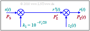
The figure shows a time domain model, with the help of which the path loss $V_{\rm P}$ can be simulated according to the above equation. Please note:
- The input signal $s(t)$ possess the power $P_{\rm S}$. In logarithmic representation, the power is related to $1\ \rm mW$ and the pseudo unit "dBm" is added.
- The path loss $V_1$ is generated by multiplication with $k_1$ The output signal $r'(t)$ then has a power that is smaller by $V_1$ (in dB) :
- \[k_1 = 10^{-V_{\rm 1}/20} \hspace{0.1cm} \Rightarrow \hspace{0.1cm} 10 \cdot {\rm lg} \hspace{0.1cm} \frac{P_{\rm E}\hspace{0.05cm}' }{\rm 1\,mW}= 10 \cdot {\rm lg} \hspace{0.1cm} \frac{P_{\rm S} }{\rm 1\,mW} + 20 \cdot {\rm lg} \hspace{0.1cm} k_1 = 10 \cdot {\rm lg} \hspace{0.1cm} \frac{P_{\rm S} }{\rm 1\,mW} - V_1 \hspace{0.05cm}.\]
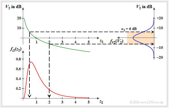
- The (mean value-free) Lognormal–Fading is simulated by multiplication with the random variable $z_2(t)$
- The PDF results from the Gaussian random quantity $V_2$ by a nonlinear Transformation at the characteristic curve
- $$z_2 = g(V_2) = 10^{-V_{\rm 2}/20}.$$
- For $z_2< 0$ this PDF is zero, and for $z_2\ge 0$ applies with the abbreviation $C = \rm ln(10)/20 dB$:
- $$f_{z_{\rm 2}}(z_{\rm 2}) = \frac {{\rm e^{- {\rm ln}^2 (z_{\rm 2}) /({2 \hspace{0.05cm}\cdot \hspace{0.05cm} C^2 \hspace{0.05cm} \cdot \hspace{0.05cm} \sigma_{\rm S}^2}) } } }{ \sqrt{2 \pi }\cdot C \cdot \sigma_{\rm S} \cdot z_2} \hspace{0.05cm}.$$
The graphic illustrates the transformation. You can see
- the Gauss–PDF of $V_2$ (blue) with scatter $\sigma_{\rm S} = 6 \ \rm dB$,
- the negative logarithmic characteristic curve (green), and
- the asymmetric PDF (red) of the size to be multiplied $z_2(t)$.
We refer here to the Exercise 1.2Z.
Requirements for the following chapters
The average power of all signal components arriving at the receiver can be calculated using path loss and shading models.
- The lognormal shadowing model takes into account slow changes of the reflectors due to the topology, with reception conditions changing only every five to ten meters in cities and every 30 to 100 meters in rural areas.
- In the following, the path loss and the influence of shadowing is not considered further, but on $1$ normalized.
Paths can overlap constructively or destructively. The associated changes occur locally in the range of half the wavelength. In mobile radio, a few centimeters are enough to find completely different reception conditions. One speaks of Fast Fading. Such a channel is basically frequency– and time-dependent.
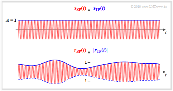
For the rest of this first main chapter, frequency dependence is eliminated by assuming a single fixed frequency (see graph).
The following conditions therefore apply with immediate effect:
- The input signal of the mobile radio channel is a cosine oscillation with the amplitude $A = 1$ and the frequency $f_{\rm T}$. We refer to this harmonic oscillation as the „transmit signal” $s_{\rm BP}(t)$. This bandpass–signal is shown in red in the upper graphic.
- The output signal $r_{\rm BP}(t)$ of the mobile radio channel – hereinafter „receive signal” called – may differ from $s_{\rm BP}(t)$ both in amplitude (envelope) and in phase ⇒ lower graph, red.
- Furthermore, we mostly look at the mobile radio channel in the equivalent low-pass range. The "transmit signal" is then $s_{\rm TP}(t) = 1$ and thus real ⇒ blue horizontal in the upper graphic.
- The LP–output signal $r_{\rm TP}(t)$ is generally complex, where the envelope is given by $a(t)$ and the phase $\phi(t)$ is noticeable by shifts in the zero crossings ⇒ blue envelope in the lower graph.
$\text{Fazit:}$ For the physical (bandpass–)signal at the output of the mobile radio channel always applies in the following:
- \[r_{\rm BP}(t) = a(t) \cdot \cos \big [2\pi f_{\rm T} t + \phi(t)\big ]\hspace{0.3cm}\Rightarrow \hspace{0.3cm} a(t) = \vert r_{\rm BP}(t)\vert\hspace{0.05cm}, \hspace{0.2cm} \phi(t) = {\rm arc}\hspace{0.15cm} r_{\rm BP}(t)\hspace{0.05cm}.\]
Exercises for the chapter
Exercise 1.1: Dual Slope Loss Model
Exercise 1.1Z: Simple Path Loss Model
Exercise 1.2: Lognormal - Channel Mode
Exercise 1.2Z: Lognormal Fading Again
Quellenverzeichnis
- ↑ 1.0 1.1 1.2 Zangl, J.: Multi-Hop-Netze mit Kanalcodierung und Medium Access Controll (/MAC). Düsseldorf: VDI Verlag, Reihe 10, Nummer 761, 2005.
- ↑ Pahlavan, K.; Allen, L.: Wireless Information Networks. New York: John Wiley & Sons, Wiley Series in Telecommunications and Signal Processing, 1995.
- ↑ Goldsmith, A.: Wireless Communications. Cambridge University Press, Cambridge, UK, 2006.
- ↑ Hindelang, T.: Mobile Communications. Vorlesungsmanuskript. Lehrstuhl für Nachrichtentechnik, Technische Universität München, 2008.
