Exercise 3.8Z: Optimal Detection Time for DFE
As in "Exercise 3.8", we consider the bipolar binary system with decision feedback equalization $\rm (DFE)$.
The pre-equalized basic pulse $g_d(t)$ at the input of the DFE corresponds to the rectangular response of a Gaussian low-pass filter with the cutoff frequency $f_{\rm G} \cdot T = 0.25$.
In the ideal DFE, a compensation pulse $g_w(t)$ is formed which is exactly equal to the input pulse $g_d(t)$ for all times $t ≥ T_{\rm D} + T_{\rm V}$, so that the following applies to the corrected basic pulse:
- $$g_k(t) \ = \ g_d(t) - g_w(t) = \ \left\{ \begin{array}{c} g_d(t) \\ 0 \\ \end{array} \right.\quad \begin{array}{*{1}c} {\rm{for}}\\ {\rm{for}} \\ \end{array} \begin{array}{*{20}c} t < T_{\rm D} + T_{\rm V}, \\ t \ge T_{\rm D} + T_{\rm V}, \\ \end{array}$$
Here $T_{\rm D}$ denotes the detection time, which is a system variable that can be optimized. $T_{\rm D} = 0$ denotes symbol detection at the pulse midpoint.
- However, for a system with DFE, $g_k(t)$ is strongly asymmetric, so a detection time $T_{\rm D} < 0$ is more favorable.
- The delay time $T_{\rm V} = T/2$ indicates that the DFE does not take effect until half a symbol duration after detection.
- However, $T_{\rm V}$ is not relevant for solving this exercise.
A low-effort realization of the DFE is possible with a delay filter, where the filter order must be at least $N = 3$ for the given basic pulse. The filter coefficients are to be selected as follows:
- $$k_1 = g_d(T_{\rm D} + T),\hspace{0.2cm}k_2 = g_d(T_{\rm D} + 2T),\hspace{0.2cm}k_3 = g_d(T_{\rm D} + 3T) \hspace{0.05cm}.$$
Notes:
- The exercise belongs to the chapter "Decision Feedback".
- Note also that decision feedback is not associated with an increase in noise power, so that an increase in (half) eye opening by a factor of $K$ simultaneously results in a signal-to-noise ratio gain of $20 \cdot {\rm lg} \, K$.
- The pre-equalized basic pulse $g_d(t)$ at the DFE input corresponds to the rectangular response of a Gaussian low-pass filter with the cutoff frequency $f_{\rm G} = 0.25/T$.
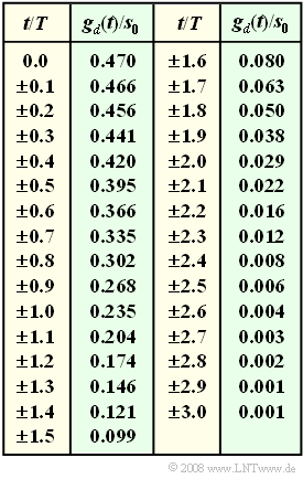
- The table shows the sample values of $g_d(t)$ normalized to $s_0$. The information section for "Exercise 3.8" shows a sketch of $g_d(t)$.
Questions
Solution
- $$\frac{\ddot{o}(T_{\rm D})}{ 2} = g_d(0) - g_d(-T)- g_d(-2T)- g_d(-3T)$$
- $$ \Rightarrow \hspace{0.3cm} \frac{\ddot{o}(T_{\rm D})}{ 2 \cdot s_0} = 0.470 - 0.235 - 0.029 -0.001 \hspace{0.15cm}\underline {= 0.205} \hspace{0.05cm}.$$
(2) The coefficients should be chosen such that $g_k(t)$ fully compensates for the trailer of $g_d(t)$:
- $$k_1 = g_d( T)\hspace{0.15cm}\underline {= 0.235},\hspace{0.2cm}k_2 = g_d(2T)\hspace{0.15cm}\underline {= 0.029},\hspace{0.2cm}k_3 = g_d(3T)\hspace{0.15cm}\underline {= 0.001} \hspace{0.05cm}.$$
(3) Based on the result of subtask (1), we obtain:
- $$\frac{\ddot{o}(T_{\rm D})}{ 2 \cdot s_0} = 0.205 - 0.5 \cdot (0.235 + 0.029 + 0.001)\hspace{0.15cm}\underline { = 0.072} \hspace{0.05cm}.$$
(4) Optimizing $T_{\rm D}$ according to the entries in the table yields:
- $$T_{\rm D}/T = 0: \hspace{0.5cm} \ddot{o}(T_{\rm D})/(2 \, s_0) = 0.470 – 0.235 – 0.029 – 0.001 = 0.205,$$
- $$T_{\rm D}/T = \ –0.1: \hspace{0.2cm} \ddot{o}(T_{\rm D})/(2 \, s_0) = 0.466 \ – \ 0.204 \ – \ 0.022 \ – \ 0.001 = 0.240,$$
- $$T_{\rm D}/T = \ –0.2: \hspace{0.2cm} \ddot{o}(T_{\rm D})/(2 \, s_0) = 0.456 \ – \ 0.174 \ – \ 0.016 \ – \ 0.001 = 0.266,$$
- $$T_{\rm D}/T = \ –0.3: \hspace{0.2cm} \ddot{o}(T_{\rm D})/(2 \, s_0) = 0.441 \ – \ 0.146 \ – \ 0.012 \ – \ 0.001 = 0.283,$$
- $${\bf {\it T}_{\rm D}/{\it T} = \ –0.4: \hspace{0.2cm} \ddot{o}({\it T}_{\rm D})/(2 \, {\it s}_0) = 0.420 \ – \ 0.121 \ – \ 0.008 \ – \ 0.001 = 0.291,}$$
- $$T_{\rm D}/T = \ –0.5: \hspace{0.2cm} \ddot{o}(T_{\rm D})/(2 \, s_0) = 0.395 \ – \ 0.099 \ – \ 0.006 \ – \ 0.001 = 0.290,$$
- $$T_{\rm D}/T = \ –0.6: \hspace{0.2cm} \ddot{o}(T_{\rm D})/(2 \, s_0) = 0.366 \ – \ 0.080 \ – \ 0.004 \ – \ 0.001 = 0.282,$$
- Thus, the optimal detection time is $T_{\rm D, \ opt} \ \underline {= \ –0.4T}$ (probably slightly larger).
- For this, the maximum value $(\underline{0.291})$ was determined for the half eye opening.
(5) With $T_{\rm D} = \ –0.4 \ T$, the filter coefficients are:
- $$k_1 = g_d(0.6 T)\hspace{0.15cm}\underline {= 0.366},\hspace{0.2cm}k_2 = g_d(1.6T)\hspace{0.15cm}\underline {= 0.080},\hspace{0.2cm}k_3 = g_d(2.6T)\hspace{0.15cm}\underline {= 0.004} \hspace{0.05cm}.$$
(6) Using the same procedure as in subtask (3), we obtain here:
- $$\frac{\ddot{o}(T_{\rm D,\hspace{0.05cm} opt})}{ 2 \cdot s_0} = 0.291 - 0.5 \cdot (0.366 + 0.080 + 0.004) \hspace{0.15cm}\underline {= 0.066} \hspace{0.05cm}.$$
The results of this exercise can be summarized as follows:
- Optimizing the detection timing ideally increases the eye opening by a factor of $0.291/0.205 = 1.42$, which corresponds to the signal-to-noise ratio gain of $20 \cdot {\rm lg} \, 1.42 \approx 3 \ \rm dB$.
- However, if the DFE functions only $50\%$ due to realization inaccuracies, then with $T_{\rm D} = \ –0.4T$ there is a degradation by the amplitude factor $0.291/0.066 \approx 4.4$ compared to the ideal DFE. For $T_{\rm D} = 0$, this factor is much smaller with $2.05/0.072 \approx 3$.
- In fact, the actually worse system $($with $T_{\rm D} = 0)$ is superior to the actually better system $($with $T_{\rm D} = \ –0.4T)$, if the decision feedback works only $50\%$. Then there is a SNR loss of $20 \cdot {\rm lg} \, (0.072/0.066) \approx 0.75 \ \rm dB$.
- One can generalize these statements: The larger the improvement by system optimization (here: the optimization of the detection time) is in the ideal case, the larger is also the degradation at non-ideal conditions, e.g., at tolerance-bounded realization.
