Exercise 1.3Z: Threshold Optimization
In this exercise, a bipolar binary system with AWGN noise ("Additive White Gaussian Noise") is considered, so that for the bit error probability:
- $$p_{\rm B} = {\rm Q} \left( \frac{s_0}{\sigma_d}\right)= {1}/{2} \cdot {\rm erfc} \left( \frac{s_0}{\sqrt{2} \cdot \sigma_d}\right) \hspace{0.05cm}.$$
Here, the following functions are used:
- $${\rm Q} (x) = \frac{\rm 1}{\sqrt{\rm 2\pi}}\int_{\it x}^{+\infty}\rm e^{\it -u^{\rm 2}/\rm 2}\,d {\it u} \hspace{0.05cm},\hspace{1cm}{\rm erfc} ({\it x}) = \frac{\rm 2}{\sqrt{\rm \pi}}\int_{\it x}^{+\infty}\rm e^{\it -u^{\rm 2}}\,d \it u \hspace{0.05cm}.$$
- The above equation holds for the threshold $E = 0$, regardless of the symbol probabilities $p_{\rm L}$ and $p_{\rm H}$.
- However, a smaller error probability can be obtained with a different threshold $E$ if the two occurrence probabilities are different $(p_{\rm L} ≠ p_{\rm H})$.
The standard deviation of the noise component is always $σ_{d} = 0.5 \ \rm V$. The two amplitudes of the detection signal component are fixed at $±1 \ \rm V$.
The following symbol probabilities are to be investigated:
- $p_{\rm L} = 0.88$ ⇒ $p_{\rm H} = 1- p_{\rm L} =0.12$,
- $p_{\rm L} = 0.31$ ⇒ $p_{\rm H} = 1- p_{\rm L} =0.69$.
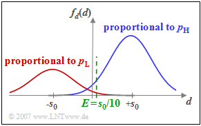
The diagram includes this last set of parameters and the threshold $E = 0.1 \cdot s_{\rm 0}$. The probability density function of the detection samples $d$ is shown.
Notes:
- The exercise belongs to the chapter "Error Probability for Baseband Transmission".
- You can use the interactive applet "Complementary Gaussian Error Functions" to determine error probabilities.
- The following applies to the derivative of the Q-function:
- $$\frac{{\rm d\hspace{0.05cm}Q} ({\it x})} {{\rm d}\hspace{0.05cm}x} = \frac{\rm 1}{\sqrt{\rm 2\pi}} \cdot \rm e^{\it -x^{\rm 2}/\rm 2} \hspace{0.05cm}.$$
Questions
Solution
- $$\rm Q (\it x)= \frac{\rm 1}{\sqrt{\rm 2\pi}}\int_{\it x}^{+\infty}\rm e^{\it -u^{\rm 2}/\rm 2}\,d \it u = \frac{\rm 1}{\sqrt{\rm \pi}}\int_{\it x/\sqrt{\rm 2}}^{+\infty}\rm e^{\it -t^{\hspace{0.05cm}\rm 2}}\,{d \it t} = {1}/{2} \cdot {\rm erfc} \left( {x}/{\sqrt{2}} \right)\hspace{0.05cm}.$$
From this it follows that the first solution is correct:
- $${\rm erfc} (x)= 2 \cdot {\rm Q} (\sqrt{2} \cdot x) \hspace{0.05cm}.$$
(2) Independently of the symbol probabilities, with the decision threshold $E = 0$, we obtain:
- $$p_{\rm B} = {\rm Q} \left( {s_0}/{\sigma_d}\right)= {\rm Q} (2) \hspace{0.1cm}\underline {= 2.27 \, \% }\hspace{0.05cm}.$$
(3) Now the general equation for the bit error probability, where $d_{\rm N}$ denotes the noise component of $d(t)$, is:
- $$p_{\rm B} \ = \ p_{\rm L} \cdot {\rm Pr}( d_{\rm N}> E + s_0)+ p_{\rm H} \cdot {\rm Pr}( d_{\rm N}< E - s_0) \ = \ p_{\rm L} \cdot {\rm Q} \left( \frac{s_0 + E}{\sigma_d}\right)+ p_{\rm H} \cdot {\rm Q} \left( \frac{s_0 - E}{\sigma_d}\right)\hspace{0.05cm}.$$
- Here, the PDF symmetry is taken into account. With $p_{\rm L} = 0.88$ ⇒ $p_{\rm H} = 0.12$ and $E = 0.1 \hspace{0.05cm} \rm V $ one obtains:
- $$p_{\rm B} \hspace{-0.05cm}=\hspace{-0.05cm} 0.88 \hspace{-0.03cm}\cdot \hspace{-0.03cm}{\rm Q} \left( \frac{1\, {\rm V} + 0.1\, {\rm V}}{0.5\, {\rm V}}\right)\hspace{-0.05cm}+\hspace{-0.05cm} 0.12 \hspace{-0.03cm}\cdot \hspace{-0.03cm}{\rm Q} \left( \frac{1\, {\rm V} - 0.1\, {\rm V}}{0.5\, {\rm V}}\right) \hspace{-0.05cm}=\hspace{-0.05cm} 0.88 \hspace{-0.03cm}\cdot \hspace{-0.03cm} {\rm Q}(2.2) \hspace{-0.05cm}+\hspace{-0.05cm} 0.12 \cdot {\rm Q}(1.8) \hspace{-0.05cm}= \hspace{-0.05cm}0.88 \hspace{-0.03cm}\cdot \hspace{-0.03cm} 1.39\,\% \hspace{-0.05cm}+\hspace{-0.05cm} 0.12 \hspace{-0.03cm}\cdot \hspace{-0.03cm} 3.59\,\%\ \hspace{0.1cm}\underline { = 1.65\,\% } \hspace{0.05cm}.$$
- Threshold shifting to the right by $E = s_{0}/10$ results in an improvement from $p_{\rm B} = 2.27 \ \%$ to $p_{\rm B} = 1.65 \ \%$.
(4) This optimization task is solved by setting the derivative to zero, taking into account the note on the information section:
- $$\frac{{\rm d\hspace{0.05cm}} p_{\rm B}(E)} {{\rm d}\hspace{0.05cm}E} = - \frac{\rm p_{\rm L}}{\sqrt{\rm 2\pi}\cdot {\sigma_d}} \cdot {\rm exp}\left(- \frac{(s_0 + E)^2}{{\rm 2}\cdot {\sigma_d}^2}\right)+\frac{\rm p_{\rm H}}{\sqrt{\rm 2\pi}\cdot {\sigma_d}} \cdot {\rm exp}\left(- \frac{(s_0 - E)^2}{{\rm 2}\cdot {\sigma_d}^2}\right) = 0$$
- $$\Rightarrow \hspace{0.3cm} \frac{p_{\rm L}} {p_{\rm H}} = - \frac{ {\rm exp} \left(-\frac{(s_0 - E)^2}{{\rm 2}\cdot {\sigma_d}^2}\right)}{{\rm exp} \left(-\frac{(s_0 + E)^2}{{\rm 2}\cdot {\sigma_d}^2}\right)} = {\rm exp} \left( \frac{2 \cdot E \cdot s_0 }{ {\sigma_d}^2}\right)\hspace{0.05cm}.$$
- Thus, we obtain for the optimal threshold value in general:
- $$E_{\rm opt} = \frac{\sigma_d^2} {2 \cdot s_0} \cdot {\rm ln}\hspace{0.05cm}\frac{p_{\rm L}} {p_{\rm H}} \hspace{0.05cm}.$$
- With $σ_{d} = 0.5 \ \rm V$, $s_{\rm 0} = 1 \ \rm V$, $p_{\rm L} = 0.88$ and $p_{\rm H} = 0.12$, the following optimum is obtained:
- $$E_{\rm opt} = \frac{(0.5\, {\rm V})^2} {2 \cdot 1\, {\rm V}} \cdot {\rm ln}\hspace{0.05cm}\frac{0.88} {0.12} \hspace{0.1cm}\underline { \approx 0.25\, {\rm V}}\hspace{0.05cm}.$$
(5) The minimum error probability for the optimal threshold $E_{\rm opt} = 0.25 \hspace{0.05cm} \rm V$ is thus:
- $$p_{\rm B, \hspace{0.05cm}min} = 0.88 \cdot {\rm Q}(2.5) + 0.12 \cdot {\rm Q}(1.5) = 0.88 \cdot 0.62\,\% + 0.12 \cdot 6.68\,\%\ \hspace{0.1cm}\underline {= 1.35\,\% }\hspace{0.05cm}.$$
- Compared to $E = 0$, the error probability is now about $40 \%$ smaller.
(6) Using the result from (4), the optimal threshold value is now:
- $$E_{\rm opt} = \frac{(0.5\, {\rm V})^2} {2 \cdot 1\, {\rm V}} \cdot {\rm ln}\hspace{0.05cm}\frac{0.31} {0.69}\hspace{0.1cm}\underline { \approx -0.1\, {\rm V}}\hspace{0.05cm}.$$
Please note:
- Because the symbol L is less probable here, the threshold must be shifted to the left – away from the more probable symbol.
- The derivation of the result for (4) and the diagram on the information section shows that the optimal threshold value is to be set exactly at the point where the two Gaussian functions intersect.
(7) Finally, using the result from (6), the following holds:
- $$p_{\rm B, \hspace{0.05cm}min} = 0.31 \cdot {\rm Q}(1.8) + 0.69 \cdot {\rm Q}(2.2) = 0.31 \cdot 3.59\,\% + 0.69 \cdot 1.39\,\%\ \hspace{0.1cm}\underline { = 2.07\,\% } \hspace{0.05cm}.$$
- Due to the less severe asymmetry, the achievable improvement of $9 \%$ is lower than calculated in subtask (5).
