Contents
- 1 Definition of the bit error probability
- 2 Definition of the bit error rate
- 3 Bit error probability and bit error rate in the BSC model
- 4 Error probability with Gaussian noise
- 5 Optimal binary receiver – "Matched Filter" realization
- 6 Optimal binary receiver – "Integrate & Dump" realization
- 7 Interpretation of the optimal receiver
- 8 Exercises for the chapter
- 9 References
Definition of the bit error probability
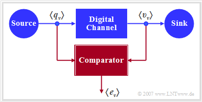
The diagram shows a very simple, but generally valid model of a binary transmission system.
This can be characterized as follows:
- Source and sink are described by the two binary sequences $〈q_ν〉$ and $〈v_ν〉$.
- The entire transmission system – consisting of
- the transmitter,
- the transmission channel including noise and
- the receiver,
is regarded as a "Black Box" with binary input and binary output.
- This "digital channel" is characterized solely by the error sequence $〈e_ν〉$.
- If the $\nu$–th bit is transmitted without errors $(v_ν = q_ν)$, $e_ν= 0$ is valid,
otherwise $(v_ν \ne q_ν)$ $e_ν= 1$ is set.
$\text{Definition:}$ The (average) bit error probability for a binary system is given as follows:
- $$p_{\rm B} = {\rm E}\big[{\rm Pr}(v_{\nu} \ne q_{\nu})\big]= \overline{ {\rm Pr}(v_{\nu} \ne q_{\nu}) } = \lim_{N \to\infty}\frac{1}{N}\cdot\sum\limits_{\nu=1}^{N}{\rm Pr}(v_{\nu} \ne q_{\nu})\hspace{0.05cm}.$$
This statistical quantity is the most important evaluation criterion of any digital system.
- The calculation as expected value $\rm E[\text{...}]$ according to the first part of the above equation corresponds to an ensemble averaging over the falsification probability ${\rm Pr}(v_{\nu} \ne q_{\nu})$ of the $\nu$–th symbol, while the line in the right part of the equation marks a time averaging.
- Both types of calculation lead – under the justified assumption of ergodic processes – to the same result, as shown in the fourth main chapter "Random Variables with Statistical Dependence" of the book "Theory of Stochastic Signals".
- The bit error probability can be determined as an expected value also from the error sequence $〈e_ν〉$, taking into account that the error quantity $e_ν$ can only take the values $0$ and $1$:
- $$\it p_{\rm B} = \rm E\big[\rm Pr(\it e_{\nu}=\rm 1)\big]= {\rm E}\big[{\it e_{\nu}}\big]\hspace{0.05cm}.$$
- The above definition of the bit error probability applies whether or not there are statistical bindings within the error sequence $〈e_ν〉$. Depending on this, one has to use different digital channel models in a system simulation. The complexity of the bit error probability calculation depends on this.
In the fifth main chapter it will be shown that the so-called "BSC model" ("Binary Symmetrical Channel") provides statistically independent errors, while for the description of bundle error channels one has to resort to the models of "Gilbert–Elliott" [Gil60][1] and of "McCullough" [McC68][2].
Definition of the bit error rate
The "bit error probability" is well suited for the design and optimization of digital systems. It is an "a–priori parameter", which allows a prediction about the error behavior of a transmission system without having to realize it already.
In contrast, to measure the quality of a realized system or in a system simulation, one must switch to the "bit error rate", which is determined by comparing the source symbol sequence $〈q_ν〉$ and the sink symbol sequence $〈v_ν〉$. This is thus an "a–posteriori parameter" of the system.
$\text{Definition:}$ The bit error rate $\rm (BER)$ is the ratio of the number $n_{\rm B}(N)$ of bit errors $(v_ν \ne q_ν)$ and the number $N$ of transmitted symbols:
- $$h_{\rm B}(N) = \frac{n_{\rm B}(N)}{N} \hspace{0.05cm}.$$
In terms of probability theory, the bit error rate is a "relative frequency"; therefore, it is also called "bit error frequency".
- The notation $h_{\rm B}(N)$ is intended to make clear that the bit error rate determined by measurement or simulation depends significantly on the parameter $N$ ⇒ the total number of transmitted or simulated symbols.
- According to the elementary laws of probability theory, only in the limiting case $N \to \infty$ the a–posteriori parameter $h_{\rm B}(N)$ coincides exactly with the a–priori parameter $p_{\rm B}$.
The connection between "probability" and "relative frequency" is clarified in the (German language) learning video
"Bernoullisches Gesetz der großen Zahlen" ⇒ "Bernoulli's law of large numbers".
Bit error probability and bit error rate in the BSC model
The following derivations are based on the BSC model ("Binary Symmetric Channel"), which is described in detail in "chapter 5.2".
- Each bit is distorted with probability $p = {\rm Pr}(v_{\nu} \ne q_{\nu}) = {\rm Pr}(e_{\nu} = 1)$, independent of the error probabilities of the neighboring symbols.
- Thus, the (average) bit error probability $p_{\rm B}$ is also equal to $p$.
Now we estimate how accurately in the BSC model the bit error probability $p_{\rm B} = p$ is approximated by the bit error rate $h_{\rm B}(N)$:
- The number of bit errors in the transmission of $N$ symbols is a discrete random quantity:
- $$n_{\rm B}(N) = \sum\limits_{\it \nu=\rm 1}^{\it N} e_{\nu} \hspace{0.2cm} \in \hspace{0.2cm} \{0, 1, \hspace{0.05cm}\text{...} \hspace{0.05cm} , N \}\hspace{0.05cm}.$$
- In the case of statistically independent errors (BSC model), $n_{\rm B}(N)$ is "binomially distributed". Consequently, mean and standard deviation of this random variable are:
- $$m_{n{\rm B}}=N \cdot p_{\rm B},\hspace{0.2cm}\sigma_{n{\rm B}}=\sqrt{N\cdot p_{\rm B}\cdot (\rm 1- \it p_{\rm B})}\hspace{0.05cm}.$$
- Therefore, for mean and standard deviation of the bit error rate $h_{\rm B}(N)= n_{\rm B}(N)/N$ holds\[m_{h{\rm B}}= \frac{m_{n{\rm B}}}{N} = p_{\rm B}\hspace{0.05cm},\hspace{0.2cm}\sigma_{h{\rm B}}= \frac{\sigma_{n{\rm B}}}{N}= \sqrt{\frac{ p_{\rm B}\cdot (\rm 1- \it p_{\rm B})}{N}}\hspace{0.05cm}.\]
- However, according to "Moivre" and "Laplace": The binomial distribution can be approximated by a Gaussian distribution:
- $$f_{h{\rm B}}({h_{\rm B}}) \approx \frac{1}{\sqrt{2\pi}\cdot\sigma_{h{\rm B}}}\cdot {\rm e}^{-(h_{\rm B}-p_{\rm B})^2/(2 \hspace{0.05cm}\cdot \hspace{0.05cm}\sigma_{h{\rm B}}^2)}.$$
- Using the "Gaussian error integral" ${\rm Q}(x)$, the probability $p_\varepsilon$ can be calculated that the bit error rate $h_{\rm B}(N)$ determined by simulation/measurement over $N$ symbols differs in magnitude by less than a value $\varepsilon$ from the actual bit error probability $p_{\rm B}$:
- $$p_{\varepsilon}= {\rm Pr} \left( |h_{\rm B}(N) - p_{\rm B}| < \varepsilon \right) = 1 -2 \cdot {\rm Q} \left( \frac{\varepsilon}{\sigma_{h{\rm B}}} \right)= 1 -2 \cdot {\rm Q} \left( \frac{\varepsilon \cdot \sqrt{N}}{\sqrt{p_{\rm B} \cdot (1-p_{\rm B})}} \right)\hspace{0.05cm}.$$
$\text{Conclusion:}$ This result can be interpreted as follows:
- If one performs an infinite number of test series over $N$ symbols each, the mean value $m_{h{\rm B} }$ is actually equal to the sought error probability $p_{\rm B}$.
- With a single test series, on the other hand, one will only obtain an approximation, whereby the respective deviation from the nominal value is Gaussian distributed with several test series.
$\text{Example 1:}$ The bit error probability $p_{\rm B}= 10^{-3}$ is given and it is known that the bit errors are statistically independent.
- If we now make a large number of test series with $N= 10^{5}$ symbols each, the respective results $h_{\rm B}(N)$ will vary around the nominal value $10^{-3}$ according to a Gaussian distribution. The standard deviation here is $\sigma_{h{\rm B} }= \sqrt{ { p_{\rm B}\cdot (\rm 1- \it p_{\rm B})}/{N} }\approx 10^{-4}\hspace{0.05cm}.$
- Thus, the probability that the relative frequency will have a value between $0.9 \cdot 10^{-3}$ and $1.1 \cdot 10^{-3}$ $(\varepsilon=10^{-4})$:
- $$p_{\varepsilon} = 1 - 2 \cdot {\rm Q} \left({\varepsilon}/{\sigma_{h{\rm B} } } \right )= 1 - 2 \cdot {\rm Q} (1) \approx 68.4\%.$$
- If this probability accuracy is to be increased to $95\%$, $N = 400\hspace{0.05cm}000$ symbols would be required.
Error probability with Gaussian noise
According to the "prerequisites to this chapter", we make the following assumptions:
- The detection signal at the detection times can be represented as follows:
- $$ d(\nu T) = d_{\rm S}(\nu T)+d_{\rm N}(\nu T)\hspace{0.05cm}. $$
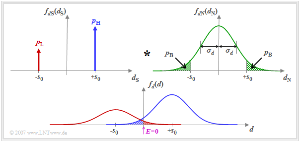
- The signal component is described by the probability density function (PDF) $f_{d{\rm S}}(d_{\rm S}) $, where we assume here different occurrence probabilities
- $$p_{\rm L} = {\rm Pr}(d_{\rm S} = -s_0),\hspace{0.5cm}p_{\rm H} = {\rm Pr}(d_{\rm S} = +s_0)= 1-p_{\rm L}.$$
- Let the probability density function $f_{d{\rm N}}(d_{\rm N})$ of the noise component be Gaussian and possess the standard deviation $\sigma_d$.
Assuming that $d_{\rm S}(\nu T)$ and $d_{\rm N}(\nu T)$ are statistically independent of each other ("signal independent noise"), the probability density function $f_d(d) $ of the detection samples $d(\nu T)$ is obtained as the convolution product
- $$f_d(d) = f_{d{\rm S}}(d_{\rm S}) \star f_{d{\rm N}}(d_{\rm N})\hspace{0.05cm}.$$
The threshold decision with threshold $E = 0$ makes a wrong decision whenever
- the symbol $\rm L$ was sent $(d_{\rm S} = -s_0)$ and $d > 0$ $($red shaded area$)$, or
- the symbol $\rm H$ was sent $(d_{\rm S} = +s_0)$ and $d < 0$ $($blue shaded area$)$.
Since the areas of the red and blue Gaussian curves add up to $1$, the sum of the red and blue shaded areas gives the bit error probability $p_{\rm B}$. The two green shaded areas in the upper probability density function $f_{d{\rm N}}(d_{\rm N})$ are – each separately – also equal to $p_{\rm B}$.
The results illustrated by the diagram are now to be derived as formulas. We start from the equation
- $$p_{\rm B} = p_{\rm L} \cdot {\rm Pr}( v_\nu = \mathbf{H}\hspace{0.1cm}|\hspace{0.1cm} q_\nu = \mathbf{L})+ p_{\rm H} \cdot {\rm Pr}(v_\nu = \mathbf{L}\hspace{0.1cm}|\hspace{0.1cm} q_\nu = \mathbf{H})\hspace{0.05cm}.$$
- Here $p_{\rm L} $ and $p_{\rm H} $ are the source symbol probabilities. The respective second (conditional) probabilities $ {\rm Pr}( v_\nu \hspace{0.05cm}|\hspace{0.05cm} q_\nu)$ describe the interferences due to the AWGN channel. From the decision rule of the threshold decision $($with threshold $E = 0)$ also results:
- $$p_{\rm B} = p_{\rm L} \cdot {\rm Pr}( d(\nu T)>0)+ p_{\rm H} \cdot {\rm Pr}( d(\nu T)<0) =p_{\rm L} \cdot {\rm Pr}( d_{\rm N}(\nu T)>+s_0)+ p_{\rm H} \cdot {\rm Pr}( d_{\rm N}(\nu T)<-s_0) \hspace{0.05cm}.$$
- The two exceedance probabilities in the above equation are equal due to the symmetry of the Gaussian probability density function $f_{d{\rm N}}(d_{\rm N})$. It holds:
- $$p_{\rm B} = (p_{\rm L} + p_{\rm H}) \cdot {\rm Pr}( d_{\rm N}(\nu T)>s_0) = {\rm Pr}( d_{\rm N}(\nu T)>s_0)\hspace{0.05cm}.$$
- This means: For a binary system with threshold $E = 0$, the bit error probability $p_{\rm B}$ does not depend on the symbol probabilities $p_{\rm L} $ and $p_{\rm H} = 1- p_{\rm L}$.
- The probability that the AWGN noise term $d_{\rm N}$ with standard deviation $\sigma_d$ is larger than the amplitude $s_0$ of the NRZ transmission pulse is thus given by:
- $$p_{\rm B} = \int_{s_0}^{+\infty}f_{d{\rm N}}(d_{\rm N})\,{\rm d} d_{\rm N} = \frac{\rm 1}{\sqrt{2\pi} \cdot \sigma_d}\int_{ s_0}^{+\infty}{\rm e} ^{-d_{\rm N}^2/(2\sigma_d^2) }\,{\rm d} d_{\rm N}\hspace{0.05cm}.$$
- Using the complementary Gaussian error integral ${\rm Q}(x)$, the result is:
- $$p_{\rm B} = {\rm Q} \left( \frac{s_0}{\sigma_d}\right)\hspace{0.4cm}{\rm with}\hspace{0.4cm}\rm Q (\it x) = \frac{\rm 1}{\sqrt{\rm 2\pi}}\int_{\it x}^{+\infty}\rm e^{\it -u^{\rm 2}/\rm 2}\,d \it u \hspace{0.05cm}.$$
- Often – especially in the English-language literature – the comparable "complementary error function" ${\rm erfc}(x)$ is used instead of ${\rm Q}(x)$. With this applies:
- $$p_{\rm B} = {1}/{2} \cdot {\rm erfc} \left( \frac{s_0}{\sqrt{2}\cdot \sigma_d}\right)\hspace{0.4cm}{\rm with}\hspace{0.4cm} {\rm erfc} (\it x) = \frac{\rm 2}{\sqrt{\rm \pi}}\int_{\it x}^{+\infty}\rm e^{\it -u^{\rm 2}}\,d \it u \hspace{0.05cm}.$$
- Both functions can be found in formula collections in tabular form. However, you can also use our HTML 5/JavaScript applet "Complementary Gaussian Error Functions" to calculate the function values of ${\rm Q}(x)$ and $1/2 \cdot {\rm erfc}(x)$.
$\text{Example 2:}$ For the following, we assume that tables are available listing the argument of the Gaussian error functions at $0.1$ intervals.
With $s_0/\sigma_d = 4$, we obtain for the bit error probability according to the Q–function:
- $$p_{\rm B} = {\rm Q} (4) = 0.317 \cdot 10^{-4}\hspace{0.05cm}.$$
According to the second equation we get:
- $$p_{\rm B} = {1}/{2} \cdot {\rm erfc} ( {4}/{\sqrt{2} })= {1}/{2} \cdot {\rm erfc} ( 2.828)\approx {1}/{2} \cdot {\rm erfc} ( 2.8)= 0.375 \cdot 10^{-4}\hspace{0.05cm}.$$
- The first value is correct. With the second calculation method, you have to round or – even better – interpolate, which is very difficult due to the strong non-linearity of this function.
- With the given numerical values, the Q–function is therefore more suitable. Outside of exercise examples, $s_0/\sigma_d$ will usually have a "curved" value. In this case, of course, the Q–function offers no advantage over ${\rm erfc}(x)$.
Optimal binary receiver – "Matched Filter" realization
We further assume the "conditions defined in the previous section".
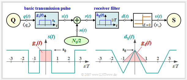
- Then we can assume for the frequency response and the impulse response of the receiver filter:
- $$H_{\rm E}(f) = {\rm sinc}(f T)\hspace{0.05cm},$$
- $$H_{\rm E}(f) \hspace{0.4cm}\bullet\!\!-\!\!\!-\!\!\!-\!\!\circ \hspace{0.4cm} h_{\rm E}(t) = \left\{ \begin{array}{c} 1/T \\ 1/(2T) \\ 0 \\ \end{array} \right.\quad \begin{array}{*{1}c} {\rm{for}} \\ {\rm{for}} \\ {\rm{for}} \\ \end{array}\begin{array}{*{20}c} |\hspace{0.05cm}t\hspace{0.05cm}|< T/2 \hspace{0.05cm},\\ |\hspace{0.05cm}t\hspace{0.05cm}|= T/2 \hspace{0.05cm},\\ |\hspace{0.05cm}t\hspace{0.05cm}|>T/2 \hspace{0.05cm}. \\ \end{array}$$
- Because of linearity, it can be written for the signal component of the detection signal $d(t)$:
- $$d_{\rm S}(t) = \sum_{(\nu)} a_\nu \cdot g_d ( t - \nu \cdot T)\hspace{0.2cm}{\rm with}\hspace{0.2cm}g_d(t) = g_s(t) \star h_{\rm E}(t) \hspace{0.05cm}.$$
- Convolution of two rectangles of equal width $T$ and height $s_0$ yields a triangular detection pulse $g_d(t)$ with $g_d(t = 0) = s_0$.
- Because of $g_d(|t| \ge T/2) = 0$, the system is free of intersymbol interference ⇒ $d_{\rm S}(\nu T)= \pm s_0$.
- The variance of the noise component $d_{\rm N}(t)$ of the detection signal ⇒ "detection noise power":
- $$\sigma _d ^2 = \frac{N_0 }{2} \cdot \int_{ - \infty }^{ + \infty } {\left| {H_{\rm E}( f )} \right|^2 \hspace{0.1cm}{\rm{d}}f} = \frac{N_0 }{2} \cdot \int_{- \infty }^{+ \infty } {\rm sinc}^2(f T)\hspace{0.1cm}{\rm{d}}f = \frac{N_0 }{2T} \hspace{0.05cm}.$$
- This gives the two equivalent equations for the bit error probability corresponding to the last section:
- $$p_{\rm B} = {\rm Q} \left( \sqrt{\frac{2 \cdot s_0^2 \cdot T}{N_0}}\right)= {\rm Q} \left( \sqrt{\rho_d}\right)\hspace{0.05cm},\hspace{0.5cm} p_{\rm B} = {1}/{2} \cdot {\rm erfc} \left( \sqrt{{ s_0^2 \cdot T}/{N_0}}\right)= {1}/{2}\cdot {\rm erfc}\left( \sqrt{{\rho_d}/{2}}\right) \hspace{0.05cm}.$$
$\text{Definition:}$ Used in this equation is the instantaneous signal–to–noise power ratio $\rm (SNR)$ $\rho_d$ of the detection signal $d(t)$ at times $\nu T$:
- $$\rho_d = \frac{d_{\rm S}^2(\nu T)}{ {\rm E}\big[d_{\rm N}^2(\nu T)\big ]}= {s_0^2}/{\sigma _d ^2} \hspace{0.05cm}.$$
In part, we use for $\rho_d$ in short the designation "detection SNR":
A comparison of this result with the section "Optimization Criterion of Matched Filter" in the book "Theory of Stochastic Signals" shows that the receiver filter
$H_{\rm E}(f)$ is a matched filter adapted to the basic transmitter pulse $g_s(t)$:
- $$H_{\rm E}(f) = H_{\rm MF}(f) = K_{\rm MF}\cdot G_s^*(f)\hspace{0.05cm}.$$
Compared to the "matched filter optimization" section, the following modifications are considered here:
- The matched filter constant is here set to $K_{\rm MF} = 1/(s_0 \cdot T)$. Thus the frequency response $ H_{\rm MF}(f)$ is dimensionless.
- The in general freely selectable detection time is chosen here to $T_{\rm D} = 0$. However, this results in an acausal filter.
- The detection SNR can be represented for any basic transmitter pulse $g_s(t)$ with spectrum $G_s(f)$ as follows, where the right identity results from "Parseval's theorem":
- $$\rho_d = \frac{2 \cdot E_{\rm B}}{N_0}\hspace{0.4cm}{\rm with}\hspace{0.4cm} E_{\rm B} = \int^{+\infty} _{-\infty} g_s^2(t)\,{\rm d}t = \int^{+\infty} _{-\infty} |G_s(f)|^2\,{\rm d}f\hspace{0.05cm}.$$
- $E_{\rm B}$ is often referred to as "energy per bit" and $E_{\rm B}/N_0$ – incorrectly – as $\rm SNR$. Indeed, as can be seen from the last equation, for binary baseband transmission $E_{\rm B}/N_0$ differs from the detection SNR $\rho_d$ by a factor of $2$.
$\text{Conclusion:}$ The bit error probability of the optimal binary receiver with bipolar signaling derived here can thus also be written as follows:
- $$p_{\rm B} = {\rm Q} \left( \sqrt{ {2 \cdot E_{\rm B} }/{N_0} }\right)= {1}/{2} \cdot{\rm erfc} \left( \sqrt{ {E_{\rm B} }/{N_0} }\right) \hspace{0.05cm}.$$
This equation is valid for the realization with matched filter as well as for the realization form "Integrate & Dump" (see next section).
For clarification of the topic discussed here, we refer to our HTML 5/JavaScript applet "Matched Filter Properties".
Optimal binary receiver – "Integrate & Dump" realization
For rectangular NRZ transmission pulses, the matched filter can also be implemented as an integrator $($in each case over a symbol duration $T)$. Thus, the following applies to the detection signal at the detection times:
- $$d(\nu \cdot T + T/2) = \frac {1}{T} \cdot \int^{\nu \cdot T + T/2} _{\nu \cdot T - T/2} r(t)\,{\rm d}t \hspace{0.05cm}.$$
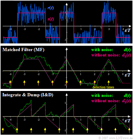
The diagram illustrates the differences in the realization of the optimal binary receiver
- with matched filter $\rm (MF)$ ⇒ middle figure, and
- as "Integrate & Dump" $\rm (I\&D)$ ⇒ bottom figure.
One can see from these signal waveforms:
- The signal component $d_{\rm S}(t)$ of the detection signal at the detection times ⇒ yellow markers $\rm (MF$: at $\nu \cdot T$, $\rm I\&D$: at $\nu \cdot T +T/2)$ is equal to $\pm s_0$ in both cases.
- The different detection times are due to the fact that the matched filter was assumed to be acausal (see last section), in contrast to "Integrate & Dump".
- For the matched filter receiver, the variance of the detection noise component is the same at all times $t$: ${\rm E}\big[d_{\rm N}^2(t)\big]= {\sigma _d ^2} = {\rm const.}$ In contrast, for the I&D receiver, the variance increases from symbol start to symbol end.
- At the times marked in yellow, the detection noise power is the same in both cases, resulting in the same bit error probability. With $E_{\rm B} = s_0^2 \cdot T$ holds again:
- $$\sigma _d ^2 = \frac{N_0}{2} \cdot \int_{- \infty }^{ +\infty } {\rm sinc}^2(f T)\hspace{0.1cm}{\rm{d}}f = \frac{N_0}{2T} $$
- $$\Rightarrow \hspace{0.3cm} p_{\rm B} = {\rm Q} \left( \sqrt{ s_0^2 / \sigma _d ^2} \right)= {\rm Q} \left( \sqrt{{2 \cdot E_{\rm B}}/{N_0}}\right) .$$
Interpretation of the optimal receiver
In this section, it is shown that the smallest possible bit error probability can be achieved with a receiver consisting of a linear receiver filter and a nonlinear decision:
- $$ p_{\rm B, \hspace{0.05cm}min} = {\rm Q} \left( \sqrt{{2 \cdot E_{\rm B}}/{N_0}}\right) = {1}/{2} \cdot {\rm erfc} \left( \sqrt{{ E_{\rm B}}/{N_0}}\right) \hspace{0.05cm}.$$
The resulting configuration is a special case of the so-called maximum a–posteriori receiver $\rm (MAP)$, which is discussed in the section "Optimal Receiver Strategies" in the third main chapter of this book.
However, for the above equation to be valid, a number of conditions must be met:
- The transmitted signal $s(t)$ is binary as well as bipolar (antipodal) and has the (average) energy $E_{\rm B}$ per bit. The (average) transmitted power is therefore $E_{\rm B}/T$.
- An AWGN channel ("Additive White Gaussian Noise") with constant (one-sided) noise power density $N_0$ is present.
- The receiver filter $H_{\rm E}(f)$ is matched as best as possible to the spectrum $G_s(f)$ of basic transmitter pulse according to the "matched filter criterion".
- The decision (threshold, detection times) is optimal. A causal realization of the matched filter can be compensated by shifting the detection timing.
- The above equation is valid independent of the basic transmitter pulse $g_s(t)$. Only the energy $E_{\rm B}$ spent for the transmission of a binary symbol is decisive for the bit error probability $p_{\rm B}$ in addition to the noise power density $N_0$.
- A prerequisite for the applicability of the above equation is that the detection of a symbol is not interfered with by other symbols. Such "intersymbol interferences" increase the bit error probability $p_{\rm B}$ enormously.
- If the absolute duration $T_{\rm S}$ of the basic transmitter pulse is less than or equal to the symbol spacing $T$, the above equation is always applicable if the matched filter criterion is fulfilled.
- The equation is also valid for Nyquist systems where $T_{\rm S} > T$ holds, but intersymbol interference does not occur due to equidistant zero crossings of the basic detection pulse $g_d(t)$. We will deal with this in the next chapter.
Exercises for the chapter
Exercise 1.2Z: Bit Error Measurement
Exercise 1.3: Rectangular Functions for Transmitter and Receiver
Exercise 1.3Z: Threshold Optimization
References


